
This is a post that I have wanted to write for a long time, but it is only now that I have the time, the disposition, and the appropriate mental state to share my ideas and knowledge on this subject. In this publication, I will try to explain what I consider to be the two main methods for analyzing circuits with alternating current (AC) power sources: Laplace Transform and Complex Frequency.
This is a somewhat lengthy post given the number of concepts that I must define before getting into the substance. Afterwards, in separate publications, I will focus on AC analysis techniques, specifically mesh analysis, nodal analysis, and possibly matrix analysis.
Before getting into the substance, I would like to clarify that this post will present important mathematical complexity. As an engineer, my strength has never been algebra or mathematics in general, but rather the application of different types of mathematical models to describe the behavior of all kinds of physical phenomena.
To solve the equations, I will use the TI-Nspire CX CAS simulator, one of the Texas Instruments calculators. This machine accompanied me during my undergraduate studies, in my master’s degree, and now in my doctoral degree. My faithful companion.
That said, let’s begin.
The excitation function
The times that I have had to teach the Circuit II course at the Technological University of Panama, I have started by explaining the concept of the excitation function. This is a mathematical model that allows us to describe any type of power source, whether voltage or current, in an electric circuit. For me, understanding this concept is fundamental.
The mathematical model is as follows:
![]()
Where:
-
- v(t) is the value of the excitation function at any time
- Vm is the maximum amplitude of the function
- t is time in seconds
- σ is the neperian frequency, given in nepers per second
- ω is the angular frequency, given in radians per second
- φ is the phase angle of the function, given in degrees
By modifying these parameters, it is possible to construct any waveform used in electrical circuits, either as voltage sources or current sources. For example:
If we consider that σ=0, ω=0 and φ=0, we will have a constant function, such as that of direct current (DC) power sources
![]()
If we consider that σ≠0, ω=0 and φ=0, we will have an exponential function:
![]()
If we consider that σ=0, ω≠0 and φ≠0, we will have a cosine function:
![]()
The excitation function is a sinusoidal function that can be damped by having non-zero values for both frequencies of the function. It’s worth noting that a cosine function can be transformed into a sine function by modifying the value of φ (specifically with a phase shift of 90º).
When I talk about this topic with my students, I like to ask them: how do we model square wave functions, sawtooth waves or similar functions? Well, for that in engineering we study a procedure that allows us to model periodic functions as a sum of sinusoidal functions: the Fourier Series.
For instance, let’s say we want to create a mathematical model that reproduces the following signal:
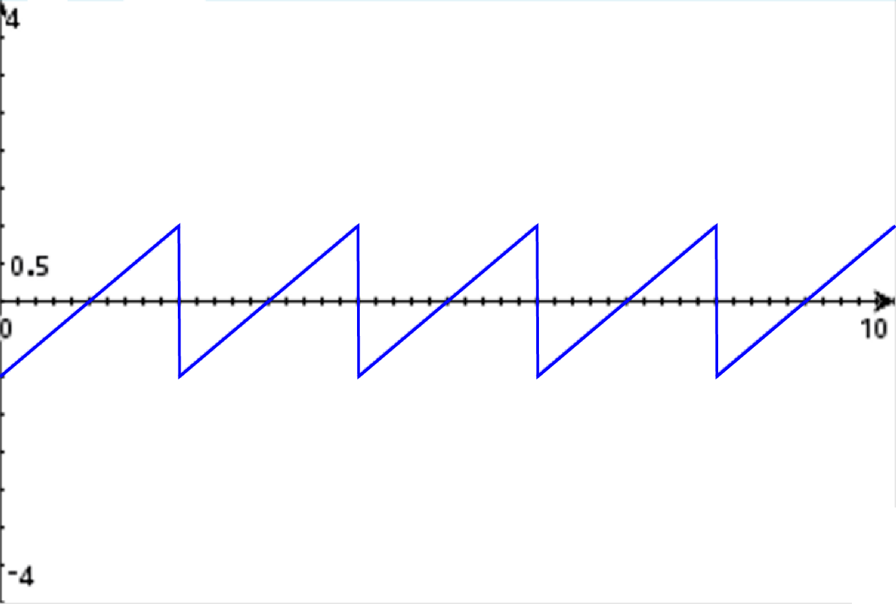
It is a sawtooth signal. The Fourier Series allows us to construct a signal like that from sines and cosines, using the following mathematical model:
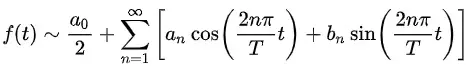 Where:
![]()
If we use this model to model the sawtooth signal shown above, the process would be:
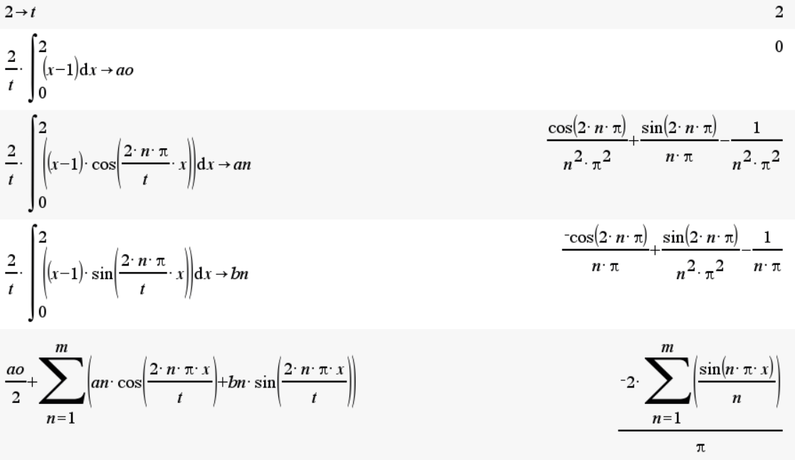
If we assign a value to the “m” of the sum, we are indicating how many harmonics we want to produce. This is known as the expansion of the Fourier Series. When we expand the series, what we get is a sum of sines and cosines:
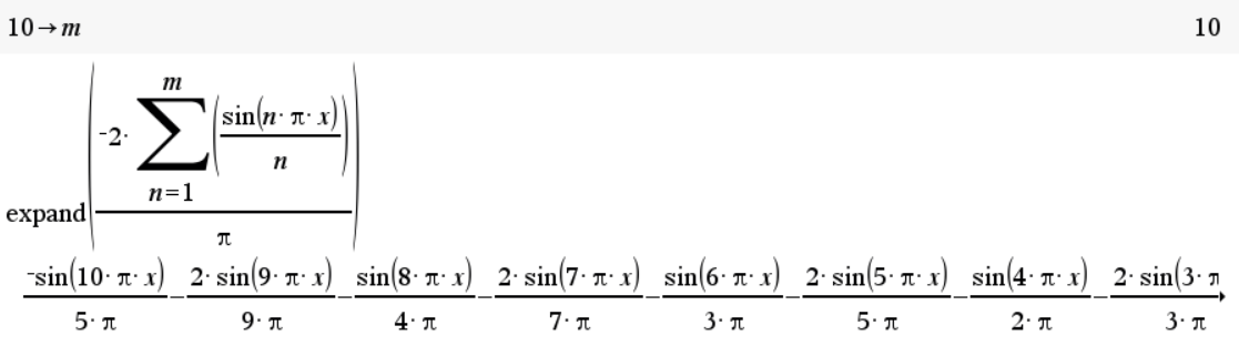
As we see, we have specified that we want an expansion of 10 harmonics. The result of the expansion is 10 sinusoidal functions, which fit the general model of the excitation function that we have presented here. If we plot the expansion of the Fourier Series, the result is:
As we can see, adding more harmonics to the expansion of the Fourier Series allows the mathematical model to gradually become more accurate in representing the sawtooth wave we wanted to model initially. The more harmonics that are used, the closer the waveform will be to the desired shape.
Regardless of the number of harmonics needed, with the excitation function (or the sum of functions) we can describe any periodic wave. We can also model non-periodic waves, using unit step functions or playing with the neperian frequency of the mathematical model.
Regardless, it is imperative to understand the excitation function and its importance in the analysis of electrical circuits.
Integro-differential equation system
What makes the analysis of AC electrical circuits difficult is not the excitation function, but the presence of reactive elements, specifically inductors and capacitors.
For example, suppose we have the following electrical circuit:
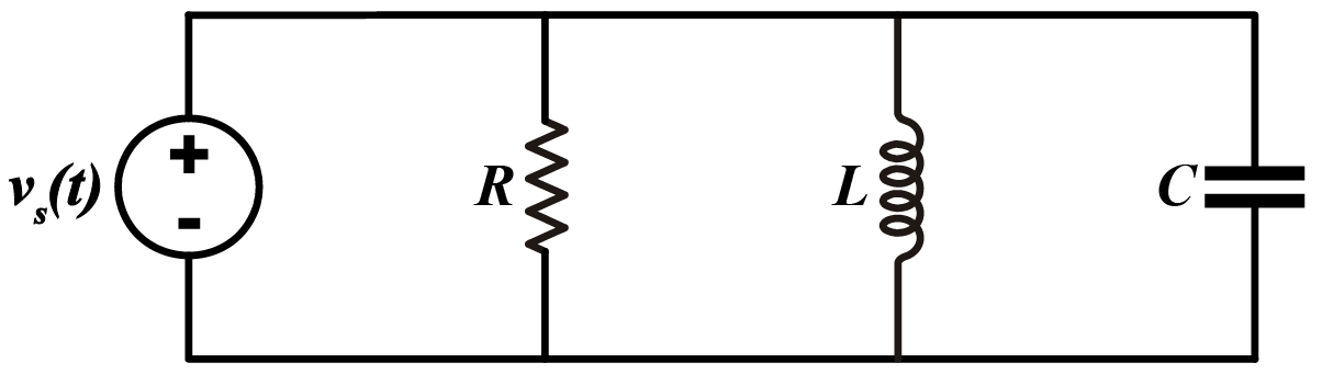
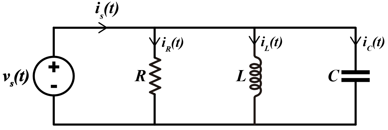
Suppose we want to know the current delivered by the power source vs(t) in the time domain. According to Kirchhoff’s Current Law, this current will be the sum of the 3 currents, the one from the resistor, the inductor, and the capacitor. This can be expressed as follows:
![]()
In the case of the resistor, the current can be easily calculated using Ohm’s Law. In the case of the inductor and the capacitor, each has a mathematical model for calculating current as a function of time.

Since the three elements are connected in parallel to the power source, the voltage at each element will be equal to the voltage of the power source. With that said, the current delivered by the power source is defined as:
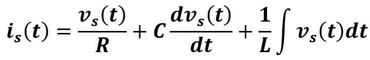
This is an integro-differential equation, that is, with integrals and derivatives in the same expression. For a mathematician, it probably isn’t very difficult to solve the derivative and integral in this expression and get the expression that represents the current delivered by the source. In engineering, you are taught to work with this type of expressions in a course called Ordinary and Differential Equations. From this point of view, the problem doesn’t seem so complicated.
However, what happens when we need to find the answer to multiple unknowns? A system of simultaneous integro-differential equations? That is precisely the problem we face when analyzing electrical circuits with multiple meshes, multiple nodes, and multiple power sources.
Transformation of mathematical models from the time domain to the frequency domain
When we have mathematical expressions that are difficult to solve in the time domain, it is very convenient to work in the frequency domain. Essentially, what we do is apply the Laplace Transform to the mathematical models in terms of time for each of the elements. Then we move on to solve the algebra in the frequency domain, and finally return to the time domain, either with an Inverse Laplace Transform or with an approximate method such as Complex Frequency.
There are other options for AC circuit analysis, such as the Fourier Transform, but in this post we will focus on the previously mentioned methods: Complex Frequency and Laplace Transform.
When working with the Laplace Transform, we often use a table of transforms to convert different types of mathematical models in the time domain to their equivalent in the frequency domain. In circuit analysis, the transforms we use most often are:
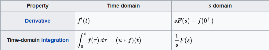
As we can see, derivatives are transformed into “s” and integrals into “1/s”. In this way, it is very easy to do circuit analysis, since it is no longer necessary to deal with integrals or derivatives. In both cases there are terms associated with the initial conditions of the circuit, but in this post we will consider that the inductors and capacitors are discharged. Later I hope to make a post in which I will explain the procedure used to analyze circuits with initial load conditions.
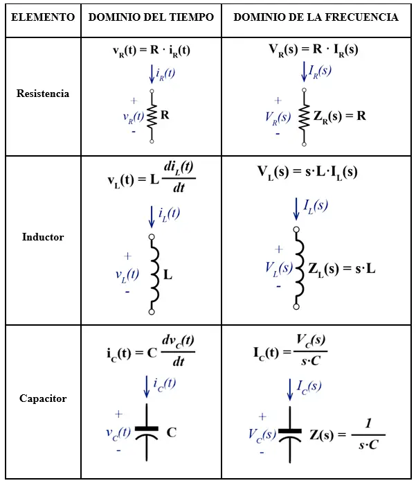
In the following table I am sharing with you the mathematical models for the resistance, inductor and capacitor in the time domain and their equivalent in the frequency domain.
I think the best way to illustrate the use of this table is by solving an example. Let’s go.
Circuit analysis in the frequency domain
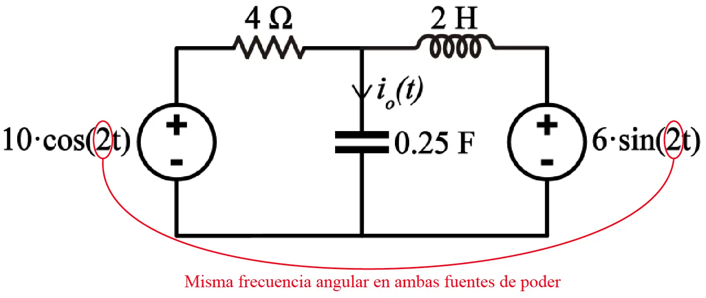
Análisis de circuitos en el dominio de la frecuencia con el siguiente circuito:
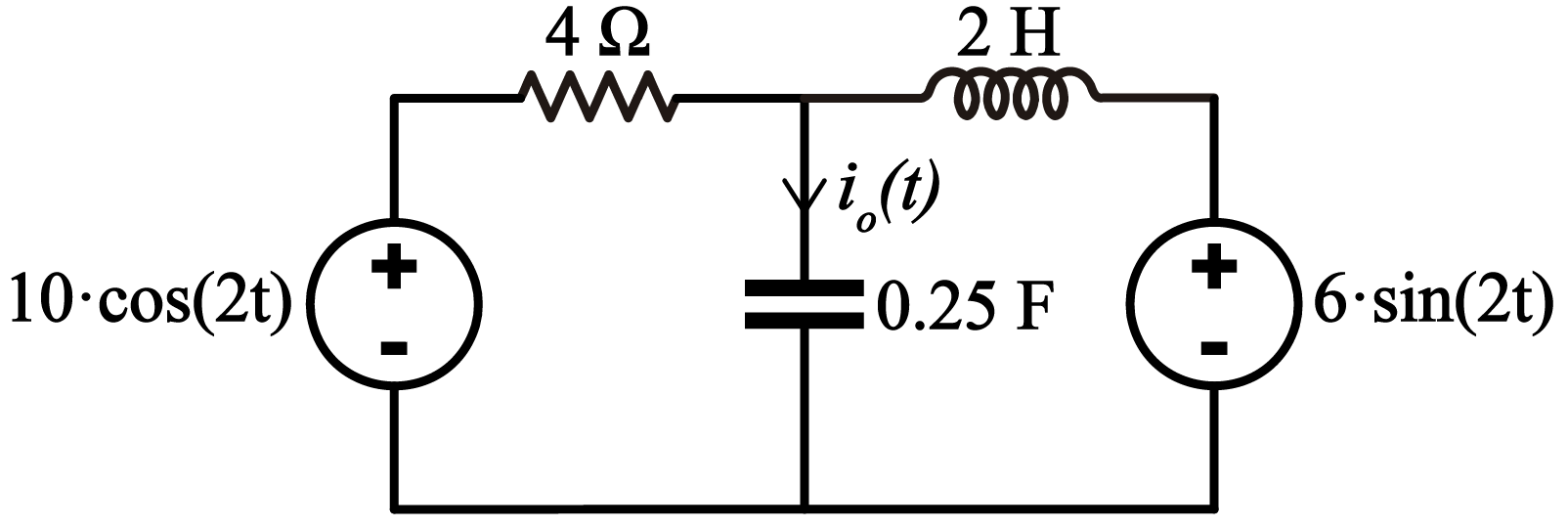
A simple circuit with two power sources, in which we have to find the current io(t). Next, I will describe the steps that in my opinion should be followed to analyze this circuit.
The first step for me is to convert the impedances and power sources to the frequency domain. To convert the impedances we use the table from the previous section. We do not apply Laplace Transform to the power sources, but instead we convert them to the frequency domain in the following way:
![]()
Note that in the time domain we use v (lowercase) and in the frequency domain we use V (uppercase). The reason for keeping the power sources as variables will be explained later. That said, our circuit converted to the frequency domain would look like this:
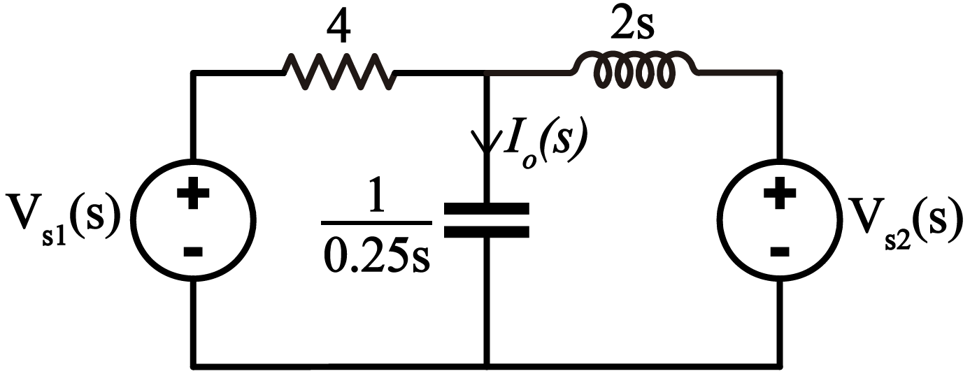
The resistance remains at 4. The inductance becomes an impedance represented by 2s and the capacitor becomes an impedance represented by 1/0.25s. This transformation has been made according to what is shown in the table in the previous section. The power sources are expressed as variables in the frequency domain.
Once the circuit is converted to the frequency domain, the techniques for analyzing circuits are used, either mesh analysis, node analysis, or any other analysis method based on Ohm’s Law. In my case, I will use node analysis to construct the following system of equations:
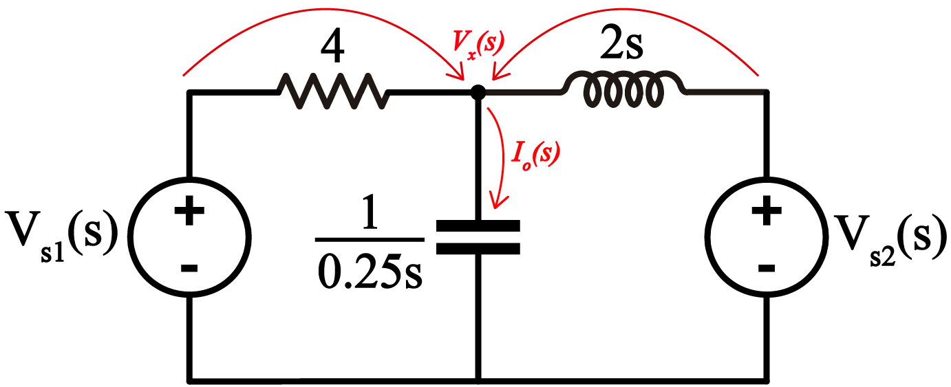
Now we sum the two currents that enter the node I have named Vx(s) and equate it to the current Io(s). Then define the current Io(s) as the voltage Vx(s) divided by the impedance of the capacitor.
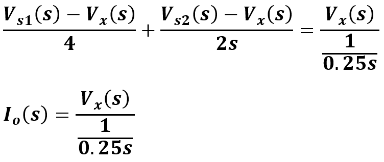
This system of equations has been defined based on Ohm’s Law and Kirchhoff’s Current Law.
This system of equations has two unknowns: Io(s) and Vx(s). Using the calculator, I will solve the system of equations:
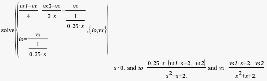
This way, the expression for Io(s) in the frequency domain is:
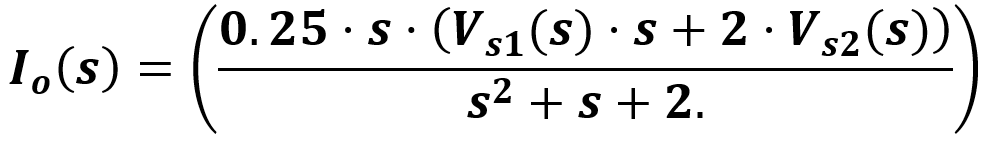
At this point, we need the expression for io(t). So far, we have Io(s). At this point, we have to decide on the type of procedure we will use to express the response, either the Inverse Laplace Transform or the Complex Frequency method.
Here is the importance of leaving the sources expressed as Vs1(s) and Vs2(s) because, as we will see below, we will be able to use the two methods we are discussing to find the solution to the problem without having to recalculate everything from the beginning.
Inverse Laplace Transform
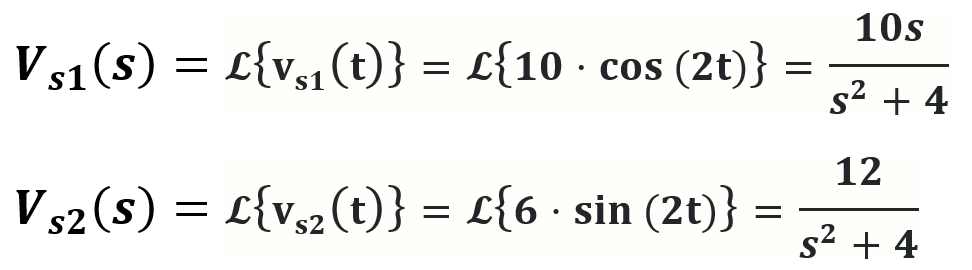
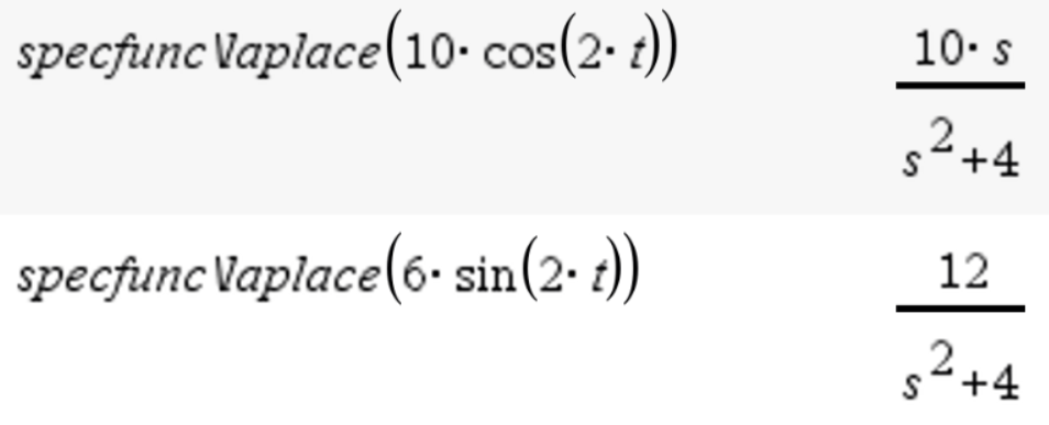
To apply the Inverse Laplace Transform it is necessary to assign a value to the power sources Vs1(s) and Vs2(s) using the Laplace Transform of Vs1(t) and Vs2(t).
These operations can be done with the Ti-Nspire CX CAS calculator:
Now we replace these expressions in the expression Io(s) that we defined in the previous section:
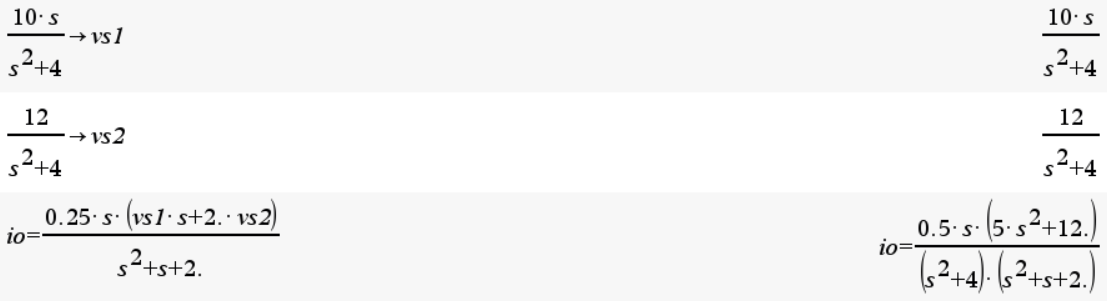
This polynomial can be broken down into smaller polynomials through the method of partial fractions. This should allow for the formation of polynomials that can be converted to the frequency domain through a table of Inverse Laplace Transforms.

This step is not necessary for me, because I have a calculator that allows me to directly do the inverse Laplace transform:
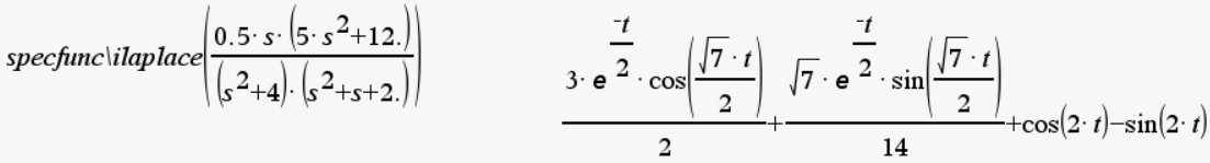
This would be the final expression for io(t), which I present adjusted below:
This would be the answer to the problem. This mathematical model describes the current io(t) at any time greater than t=0.
I must emphasize that the answer obtained with the Laplace Transform is an exact answer. As I will explain later, with the Complex Frequency method we will obtain an approximate response that will converge with the response of the Laplace Transform once the terms with exponential functions have been extinguished.
Complex frequency
The Complex Frequency method makes it possible to obtain an approximate answer to a circuit analysis problem in alternating current, without the need to use the Inverse Laplace Transform.
This method is the one normally used in Steady State Sinusoidal Analysis or phasor analysis. It is also the basis for the analysis of electrical power circuits. To apply this method, it is necessary to understand the concept of complex frequency variable.
Here it will not be necessary to do an Inverse Laplace Transform. We will simply replace the variable “s” in the polynomial Io(s) by a complex number, whose value will depend on the angular frequency (σ) and the angular frequency (ω) of the excitatory function used to power the electrical circuit.
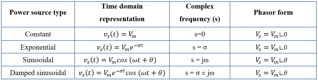
The following table presents the form that the complex frequency variable will have as a function of the frequency(s) of the excitatory function:
At the beginning of this post we invested a section in explaining the characteristics of this function.
Analyzing the original circuit, we can identify the type of exciter function of the power sources:
Both are cosine power sources. Even though the power source on the right uses the sine function, it can be converted to a cosine function with a 90º phase shift. The two sources have the same angular frequency: 2 rad/s (the number inside the parentheses that accompanies the “t”).
Taking this into account we can define our complex frequency variable:
![]()
In this expression, the “j” represents the imaginary operator, that is, square root of -1:
![]()
For mathematicians, the imaginary operator is normally represented by the letter “i”, but in Electrical Engineering it is customary to use “j” to avoid confusion with the i used to represent the intensity of electric current.
We say that “s” is the variable of complex frequency because depending on the type of exciter function this variable can be a real number (exponential source), imaginary (sinusoidal source), complex (damped sinusoidal) or zero (DC case).
Note that in order to use this method it is necessary that all power sources use the same angular frequency and natural frequency. If we had power sources with different frequencies, it would be necessary to use the superposition method, which requires special considerations for its implementation. This is a disadvantage of this method with respect to that of the Laplace Transform, which is independent of the frequency of the excitatory function(s).
Another requirement of this method is to define the power sources in their phasor form. We can see this in the table that we shared above with the types of sources, specifically in the column on the right. We need to define the power sources VS1 and VS2 as phasors:
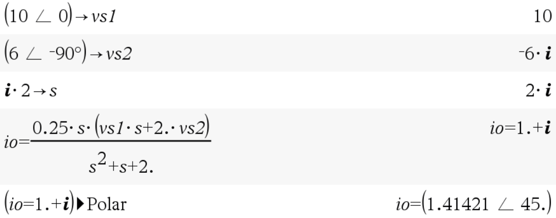
Basically what we do is take the amplitude and express it as a complex number in its polar form, whose phase angle will be the phase difference φ of the cosine function. When we have a sine function, we convert it to cosine by adding a 90º offset, which causes the phasor form to have a 90º lag.
Once the power sources have been defined in their phasor form and a value has been assigned to the complex frequency variable, we replace these values in the Io(s) expression that we left defined a while ago:
Substituting, we get the following:
The answer we got is:
![]()
Here we have the answer expressed in its rectangular form and in its polar form. From this result we can obtain an answer in the time domain:
![]()
Both answers are valid, one from the rectangular answer and the other from the polar answer. Both are equivalent, but with different notations.
If you ask me, I preferred the first answer, the rectangular answer, to avoid using offset angles with the polar answer. Using offset angles always causes inconvenience when entering data into the calculator.
Comparison of responses obtained with each method
The answer obtained with the Inverse Laplace Transform was:
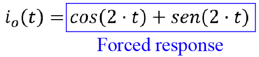
The response obtained with the Complex Frequency method was:
![]()
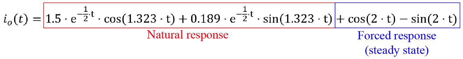
At first it seems that the answers are not the same, but in reality they are the same answer. As I mentioned before, the Inverse Laplace Transform allows us to calculate the exact answer to the problem. This response is made up of the natural response and the forced response, which in turn is the sinusoidal response in steady state.
In the case of the phasor method (Complex Frequency), the result will be the forced response, without the natural response.
The natural response occurs during circuit energization, but this will die down after some time. This is because the natural response is multiplied by an exponential function with a negative exponent. This type of function complies with the form:
![]()
In this type of functions we have a time constant, denoted by τ, which allows us to calculate the discharge time of the function. In a function of this type, the discharge time is equal to 5τ. Let’s see an example:
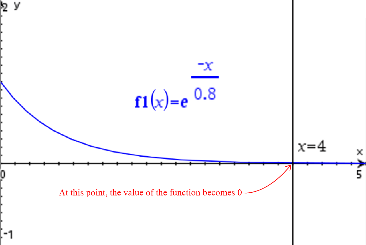
In this graph the value of τ is 0.8. The discharge time of this function will be 5×0.8=4.0. That is precisely what the graph shows.
That said, when we factor the answer obtained with the Inverse Laplace Transform we have:

The term circled in red is an exponential function with a negative exponent, such as the one shown above. The tau is 2 (τ=2), so the natural response is expected to die out after 10 seconds (5τ=10). After this time, the response obtained with the Complex Frequency method and the response obtained with the Inverse Laplace Transform will converge to the same value:
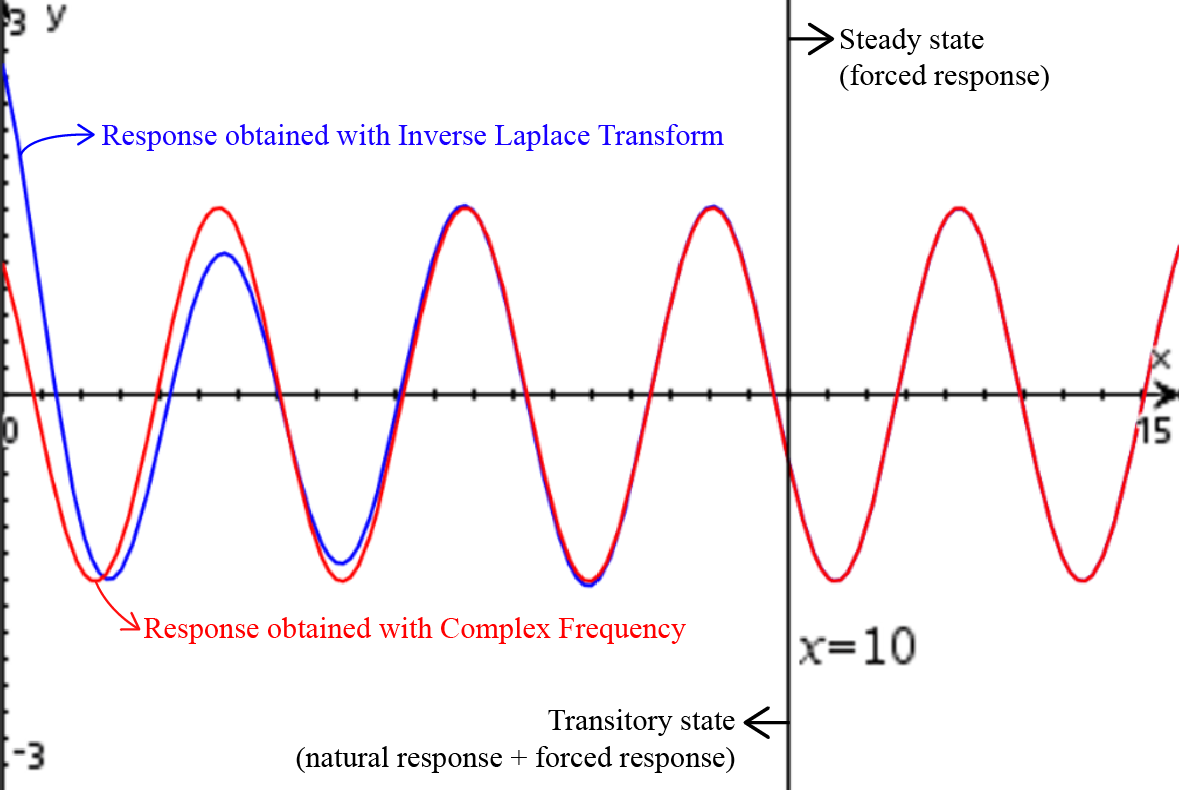
As we can see, in the initial moments of the energization of the circuit, the natural response that we calculate with the Inverse Laplace Transform can bee seen. But after the time 5τ of the exponential function of the natural response is exceeded, the responses obtained with each method of analysis converge. This is the reason why the Complex Frequency method is considered a valid analysis method, because even though it does not allow us to calculate the natural response of the circuit, it does allow us to know the response in steady state.
Advantages and disadvantages of the methods used
The Complex Frequency method allows us to obtain the steady state response of an alternating current circuit without having to deal with the Inverse Laplace Transform. Said method requires significant algebraic management, which is impractical when the necessary tools are not available to solve the mathematical problem. By representing the power sources as phasors and replacing the complex frequency variable by the corresponding complex number, it is not necessary to solve a single algebraic operation.
On the other hand, when working with Complex Frequency it is not possible to consider power sources with multiple frequencies and it is necessary to use the superposition method. This makes it especially difficult to use this technique when working with systems with harmonic content or DC components, such as in current electrical systems. The same applies to electrical circuits in which the power source must be modeled by means of a Fourier Series. Even so, the Complex Frequency method or Steady State Sinusoidal Analysis (Phasors) is the preferred method for the analysis of power systems worldwide.
The Laplace Transform is used in cases where it is imperative to know the natural response of a system, in instances where there are power sources with multiple frequencies or in systems with non-periodic disturbances. Remember that the Complex Frequency method gives us the stable response in the long term and ignoring the initial moments after a change in the excitatory function of the system.
Finally, I must highlight that in this post we have analyzed systems that are energized from a zero energy state, that is, without energy stored in the inductors and capacitors. When we have an initial charge on inductors and capacitors the Complex Frequency method becomes especially difficult to use because of all the mathematical procedures that are required to calculate the natural response. But that is a topic that I will deal with in another post later.
Conclusion
In this post I have presented a detailed explanation on the analysis of electrical circuits with time dependent power sources (and/or alternating current). Two main methods have been mentioned: the Laplace Transform and the Complex Frequency. An example of how to use these methods to analyze a circuit and obtain the response of the circuit in the time domain has been presented. The excitatory function has also been mentioned as a mathematical model that allows describing any type of power source in an electrical circuit.
I hope this post has been helpful in understanding how circuit analysis is done with time-dependent power supplies. If you have any questions or comments, I’ll be happy to answer! Thank you for reading!