
One of the most popular classification algorithms is the KNN algorithm in Machine Learning. The K-Nearest Neighbors (KNN) classifier is a simple and effective method for image and general data classification. In this article, we will explore the use of the KNN classifier on the well-known MNIST dataset of handwritten digits.
We will use the scikit-learn library in Python to train and evaluate the classifier, and we will conduct a hyperparameter search to find the best combination of parameters for the KNN model. By the end of this article, you will understand how to use the KNN classifier for image classification and how to optimize its performance through hyperparameter tuning.
Features of the K-Nearest Neighbor classifier
The K-Nearest Neighbors algorithm is a non-parametric classification method that assigns a sample a class based on the majority of the classes of its nearest neighbors in the feature space. In other words, a sample is classified according to the most common class of the K samples closest to it in the feature space. KNN is commonly used in classification and regression problems.
The value of k is determined by the user and can affect the complexity and accuracy of the model. The parameter “k” is the number of nearest neighbors that are used to make a prediction. For example, if k=3, then the algorithm will consider the 3 nearest neighbors to a sample and make a prediction based on their classes. The value of k can be chosen by the user and can affect the complexity and accuracy of the model.
A smaller value of k can lead to a model with lower bias but higher variance, while a larger value of k can lead to a model with higher bias but lower variance. In general, it is a good idea to test several values of k to see which gives the best performance on training and test data. It is also common to use odd values of k to avoid ties in class prediction.
One of the benefits of the K-Nearest Neighbors algorithm is that it has a low training time, as it does not require a complex model to fit the training data. Instead, it simply stores the training data and makes predictions based on the K nearest neighbors to a sample when asked to classify new data. This means that the training time is essentially constant, regardless of the size of the training dataset.
Despite its simplicity, KNN can still achieve high accuracy in many tasks, especially when the number of features is low and the classes are well separated. It is also a robust algorithm that is not sensitive to the scale of features or the presence of noise in the data. However, it can be sensitive to the value of K, and its performance may be compromised when the number of features is high or when the classes are not well separated.
How does the KNN algorithm work?
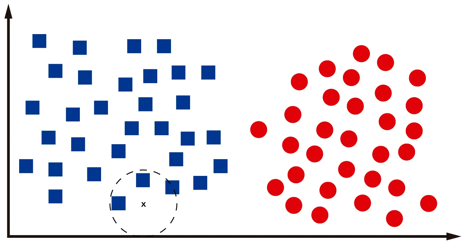
To illustrate how KNN works, I’m going to present some images with a hypothetical data classification scenario. Let’s assume we have the following dataset on some plane:
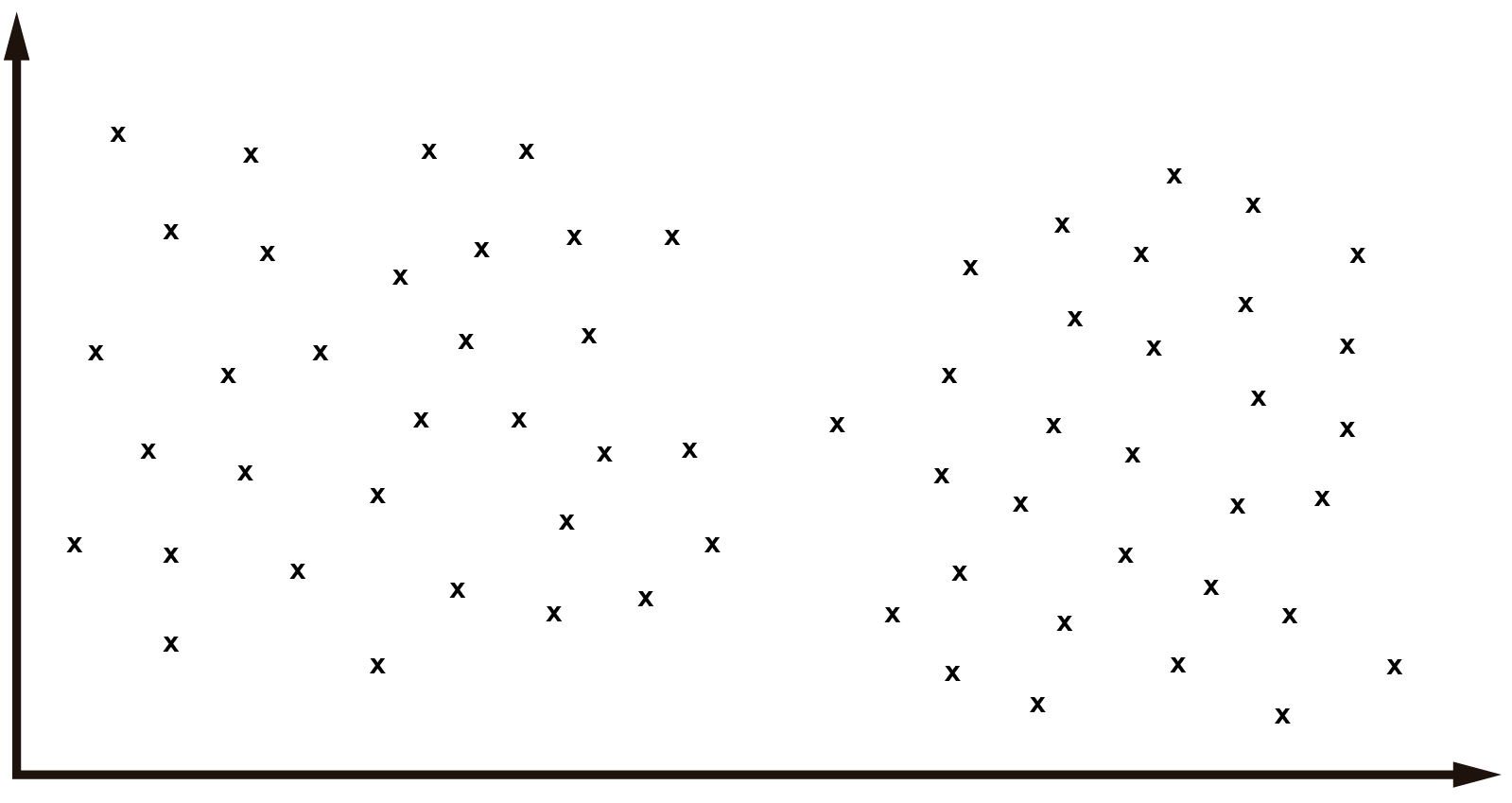
Each “x” represents a data point in the spatial plane. Now let’s assume that I, as a human, am asked to classify the data into groups. I think we can all agree that there are two main data groups, roughly separated by the horizontal plane’s midpoint.
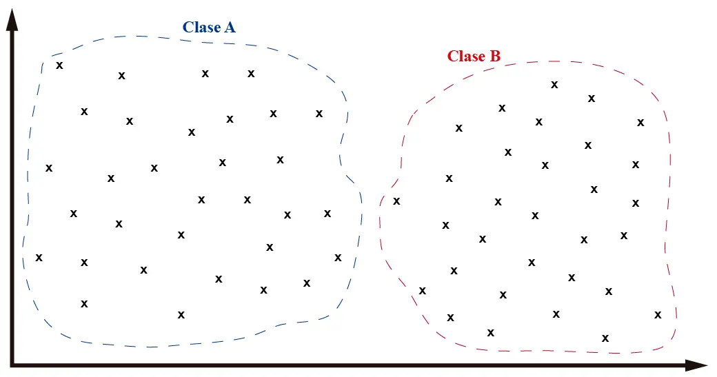
As we can see in the image, we have separated the data into two groups. In Machine Learning, when we deal with datasets, we don’t talk about groups or sets but classes. And each class can represent any object in the real world. In my case, I’ll consider that objects of “class A” are squares and objects of “class B” are circles.
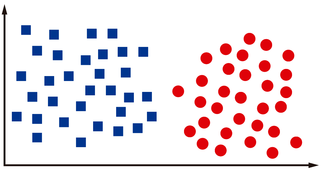
The moment I, a human, decided to classify the dataset’s objects into two classes and assigned a class to each sample, I constructed a training dataset. With this dataset, we can train a Machine Learning classifier to classify new data we haven’t seen yet.
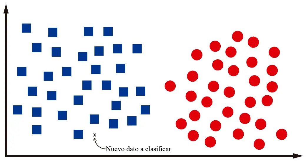
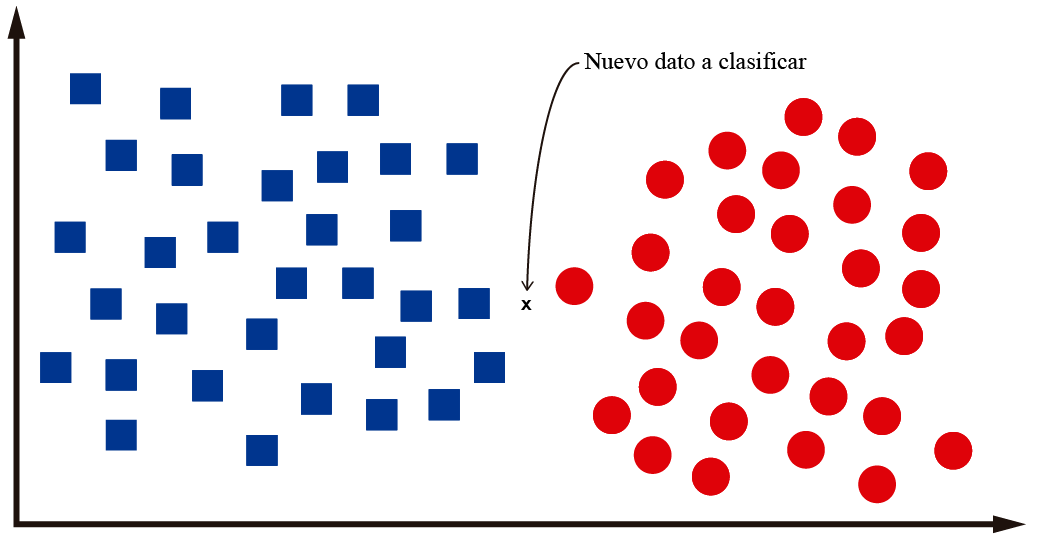
For example, let’s assume that after training our classification algorithm, we’re asked to classify a new data point:
We, as humans, can identify that this new data point is a square. That is, it’s surrounded by other squares. To classify it as a circle, it should be further to the right of the plane, where the other circles are. It’s not that hard, right?
But how do we make a computer program classify this data correctly? How do we make the computer “think” like us humans? Well, the truth is, we won’t make the computer think. But we can teach it to discriminate between squares and circles using a Machine Learning algorithm.
Each algorithm available today solves this problem differently. In KNN’s case, we’ll identify the “k” nearest neighbors to the data point we want to classify. This way, the computer can determine the data point’s proximity to the two available classes and decide whether it belongs to one or the other.
As we can see in the image, the 3 closest “neighbors” to the data point we want to classify are squares. Thus, it’s very likely that the “x” in the image represents a square. Note that I used the word “likely” because the Machine Learning paradigm is based more on probabilities than certainties.
Since this method is based on checking a data point’s “neighbors,” it’s logical that the KNN algorithm is named as such. K-Nearest Neighbors means k-closest neighbors. I think KNN is the computational representation of the saying “Tell me who you’re with, and I’ll tell you who you are.”
What happens when we need to classify data that’s located between the two classes? Let’s look at the following image:
For the data point shown in the image, it’s not easy to determine if it belongs to one class or the other. Even I, as a human, am not sure if it’s a square or a circle. For the computer, it will check the “k” nearest neighbors, calculating the distance between the neighbors’ centroids and the new data point to be classified. If we work with k=3, we’ll have something like this:
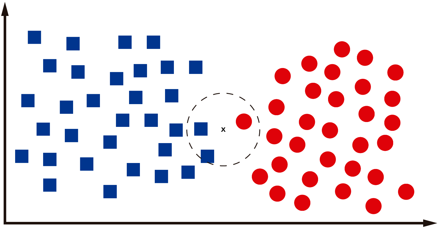
Clearly, the data point is a square, as two out of its three closest neighbors are squares. If there’s a tie, where two or more classes have the same number of occurrences among the K nearest neighbors, then the sample can be assigned to the class with the lowest index value.
This classification method is known as majority voting, as the sample’s class is determined based on the majority class among its neighbors. It’s a simple and effective method for classification and is easy to understand and implement.
Broadly speaking, this is how the KNN algorithm works. There are other important hyperparameters to consider with this algorithm, besides the number of neighbors considered in classification:
- weights: This hyperparameter controls how much weight is given to the nearest neighbors in classification, with options being ‘uniform’ (all neighbors have the same weight) or ‘distance’ (neighbors have weights proportional to the inverse of their distance).
- algorithm: This hyperparameter controls the algorithm used for the nearest neighbor search. Options include ‘brute’, which uses a brute force search, ‘kd_tree’, which uses a KD-tree data structure for faster search, and ‘ball_tree’, which uses a search tree for faster search.
- leaf_size: This hyperparameter controls the number of samples in a KD or ball tree leaf. It can affect the speed of the nearest neighbor search.
- p: This hyperparameter controls the distance metric used for the nearest neighbor search. Options include p=1 for Manhattan distance and p=2 for Euclidean distance.
In general, that’s what the KNN algorithm is about for classification in Machine Learning.
Hyperparameter Optimization
My interest in K-Nearest Neighbors arose after my previous publication in which we conducted tests with different types of classifiers on the MNIST dataset. KNN achieved a relatively high accuracy (96.82%), although it was lower than other algorithms such as Support Vector Machine (97.85%) and Random Forest (96.97%). However, there was one area where KNN proved to be one of the best:
- KNeighborsClassifier | training time: 0.18 seconds, testing time: 6.30 seconds, 96.64%
- RandomForestClassifier | training time: 46.06 seconds, testing time: 0.43 seconds, 96.97%
- SVC | training time: 167.80 seconds, testing time: 85.12 seconds, 97.85%
The training time is significantly shorter than the algorithms that achieved better performance on MNIST. This piqued my interest in this algorithm, as it’s possible that with some hyperparameter optimization, better results can be achieved.
So I wrote the following script, based on our publication about hyperparameter optimization:
|
1 2 3 4 5 6 7 8 9 10 11 12 13 14 15 16 17 18 19 20 21 22 23 24 25 26 27 28 29 30 31 32 33 34 35 36 37 38 39 40 41 42 43 44 45 46 47 48 49 |
from sklearn.model_selection import GridSearchCV import pandas as pd import numpy as np from sklearn.neighbors import KNeighborsClassifier """ Here I set the global variables, which will be used to test the computing time for both training and testing """ def loadDataset(fileName, samples): # A function for loading the data from a dataset (MNIST) x = [] # Array for data inputs y = [] # Array for labels (expected outputs) train_data = pd.read_csv(fileName) # Data has to be stored in a CSV file, separated by commas y = np.array(train_data.iloc[0:samples, 0]) # Labels column x = np.array(train_data.iloc[0:samples, 1:]) / 255 # Division by 255 is used for data normalization return x, y # Define the grid of hyperparameter values to search over param_grid = { 'n_neighbors': [3, 5, 7, 9, 11], 'weights': ['uniform', 'distance'], 'leaf_size': [5, 10, 20, 30, 35, 40, 45, 50] } # Define the scoring metric to use for evaluation scoring = 'accuracy' # Create a GridSearchCV object clf = KNeighborsClassifier() grid_search = GridSearchCV(estimator=clf, param_grid=param_grid, scoring=scoring, cv=2, verbose=2) train_x,train_y = loadDataset("../../../../datasets/mnist/mnist_train.csv",50000) test_x,test_y = loadDataset("../../../../datasets/mnist/mnist_test.csv",10000) # Fit the grid search object to the training data grid_search.fit(train_x, train_y) # Print the best hyperparameters and the best score print("Best hyperparameters:", grid_search.best_params_) print("Best score:", grid_search.best_score_) # Re-train the model with the best hyperparameters best_clf = grid_search.best_estimator_ best_clf.fit(train_x, train_y) # Test the model with the best hyperparameters on the testing data accuracy = best_clf.score(test_x, test_y) print("Testing accuracy:", accuracy) |
You can download this algorithm from our Github repository. The outcome of this algorithm should look something like this:
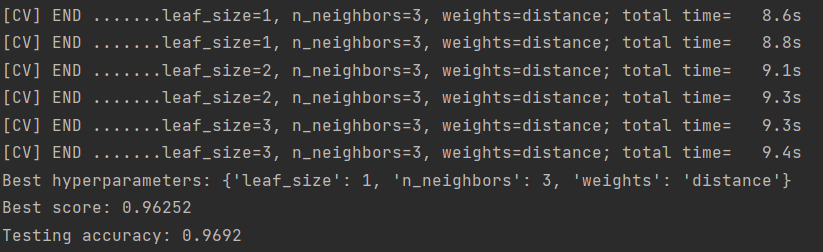
After testing various parameter combinations, we achieved a 96.92% accuracy in MNIST classification, using the parameters shown in the image.
The time each test takes is relatively short, about 9 seconds. I tested up to 200 combinations, and as I decreased the number of neighbors, I obtained better results. It is what it is.
Conclusions
In summary, in this post, we’ve explored the use of the K-Nearest Neighbors algorithm for image classification on the MNIST dataset. We’ve seen that KNN is a non-parametric classification method that has a short training time and can achieve high accuracy in many tasks. We’ve also seen how to use the scikit-learn library in Python to train and evaluate a KNN model and conduct a hyperparameter search to find the best parameter combination.
I hope you enjoyed reading this post and learned something new about using the K-Nearest Neighbors algorithm for image classification. If you have any questions or comments, please feel free to leave a message below. Thank you for reading!
Let me know if you need any further assistance!


