
Reinforcement learning is a subfield of artificial intelligence that is concerned with developing algorithms and models that can learn from feedback and optimize actions to achieve a specific goal. One popular application of reinforcement learning is training an Artificial Intelligence (AI) agent to play video games.
In this blog post, we’ll explore how to use reinforcement learning to train an AI agent to play the classic Atari game, Breakout. We’ll discuss the Deep Q-Network (DQN) algorithm, which is a popular technique for training game-playing AI agents. We’ll also provide a step-by-step tutorial on how to implement the DQN algorithm in Python using the PyTorch library and the OpenAI Gym environment to train an AI agent to play Atari Breakout.
The results of training a model with this algorithm can be seen in the following video:
By the end of this post, you’ll have a good understanding of how to use reinforcement learning to train an AI agent to master Atari games in Python. Let’s start.
What is Reinforcement Learning?
Reinforcement learning (RL) is a subfield of artificial intelligence (AI) that focuses on developing algorithms and models that enable agents to learn from feedback to optimize their actions to achieve a particular goal.
In reinforcement learning, an agent interacts with an environment and receives rewards or penalties for its actions. The agent then uses this feedback to update its decision-making process and improve its future actions to maximize the cumulative reward over time.
RL has been successfully applied in various domains such as robotics, game playing, recommendation systems, and more. The primary advantage of reinforcement learning is its ability to learn from trial-and-error without requiring a pre-defined set of rules or examples.
I don’t intend to explore this topic further in this blog post, as I’m planning to write another one that specifically covers the details of reinforcement learning. I want to make it clear that I’ll be using RL algorithms to train an AI agent to play Atari Breakout. To achieve this, we’ll create an environment where the agent can play the game, make decisions, and learn from the outcomes of those decisions. After several hours of training, the agent should be able to play the game at a high level on its own.
Algorithm composition
The following image has a visual representation of the algorithm that will be presented in this post:
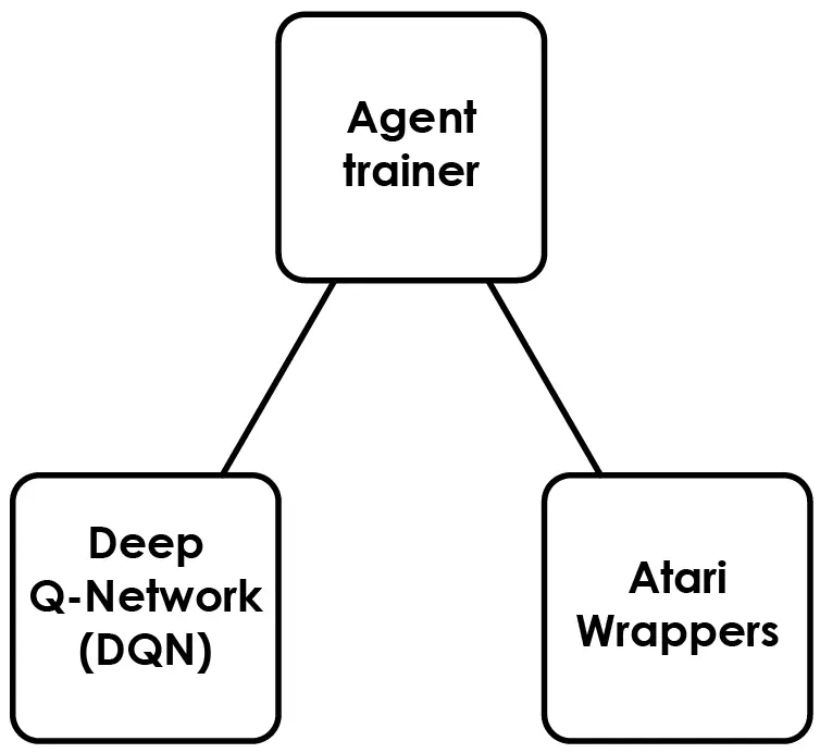
Each component has been built as a separated python script, which can be found in our Github repository. Here is a high-level description of each component:
- Deep Q-Network (DNQ): a Python script that defines the neural network architecture, epsilon-greedy action selection strategy, replay memory buffer, and a function for converting input image frames to PyTorch tensors for the Deep Q-Network (DQN) algorithm used to train an agent to play a game from pixel input.
- Agent trainer: a Python script that trains a neural network to learn how to play the game using reinforcement learning and saves the trained policy network.
- Atari Wrappers: a Python script containing a set of wrappers for modifying the behavior of Atari environments in OpenAI Gym, with the goal of preprocessing raw game screen frames and providing additional features for training reinforcement learning models
This project also includes the Renderer script, which loads a trained policy file and uses it to play the game. This allows us to observe the progress of the agent visually and evaluate its real-time performance.
Going forward, I will provide a detailed explanation of each script, allowing you to gain a better understanding of the inner workings of this algorithm.
Deep Q-Network (DNQ)
This part of the algorithm has been built in the dqn.py script. It defines the neural network architecture for the Deep Q-Network (DQN) algorithm, which is used to train an agent to play a game from pixel input. The neural network architecture consists of convolutional layers followed by fully connected layers. The agent learns to play the game using reinforcement learning by interacting with the environment and updating the weights of the neural network accordingly.
Here is a graphical representation of the neural network:
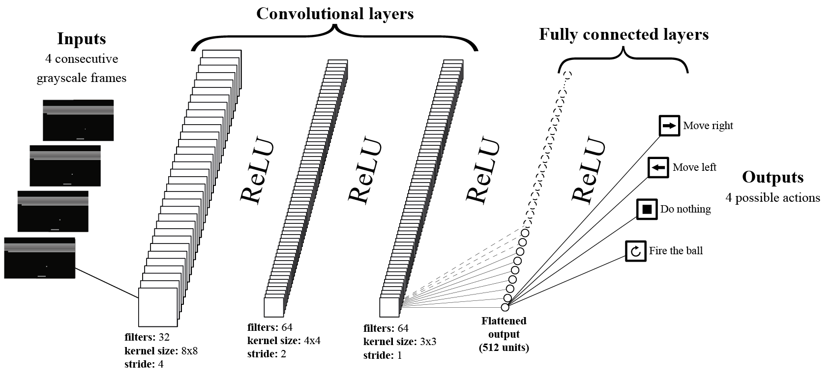
The neural network architecture takes 4 consecutive frames as input. Each frame is represented as a 3D matrix of pixels, which can be obtained using the OpenAI Gym tools. The frames are then converted to grayscale, effectively reducing the 3 dimensions of color to a single one, resulting in a 2D matrix representation.
This process is represented in the following image:
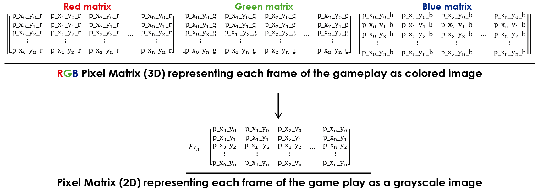
Reducing the dimensions of the input is advantageous for training the Neural Network as it reduces the amount of information to process. In this game, color is not crucial for recognizing any significant features that could aid in learning from the environment.
In the Python script, this dimension reduction is done using the fp function:
|
1 2 3 4 |
def fp(pixels): pixels = torch.from_numpy(pixels) height = pixels.shape[-2] return pixels.view(1, height, height) |
These code lines transform the image dimensions from 3 to 1 and reshape it to a square form (height by height). This compresses the image and reduces its size, leading to a minor loss of data. However, this transformation simplifies the image processing.
That said, each frame will be represented as a matrix like this:
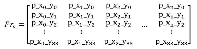
By using 4 consecutive frames of the game as input, we can provide better information about what is happening in the game. A single frame doesn’t show enough context, like whether the ball is moving up or down or how fast it’s moving.
These 4 frames are packed into a new matrix, the Frame Stack Matrix:
The Frame Stack matrix may look like a 2D matrix, but it’s actually a 3D matrix. Each index in the matrix contains a Frame matrix, which is a 2D matrix.
Finally, we will combine the 32-frame stack matrix into a “batch” matrix, which is a 4D matrix. This 4D matrix, also known as the input tensor, will be passed as input to the neural network.

When training the neural network, each element of the input tensor will be passed through the neural network, as shown in the graphical representation of the Deep-Q Learning Neural Network (see above).
The structure of the neural network is defined in the constructor of class DQN:
|
1 2 3 4 5 6 7 8 9 10 11 12 |
class DQN(nn.Module): def __init__(self, outputs, device): super(DQN, self).__init__() # Define the convolutional layers self.conv1 = nn.Conv2d(4, 32, kernel_size=8, stride=4, bias=False) self.conv2 = nn.Conv2d(32, 64, kernel_size=4, stride=2, bias=False) self.conv3 = nn.Conv2d(64, 64, kernel_size=3, stride=1, bias=False) # Define the fully connected layers self.fc1 = nn.Linear(64 * 7 * 7, 512) self.fc2 = nn.Linear(512, outputs) # Store the device where the model will be trained self.device = device |
This PyTorch Neural Network code is straightforward and easy to understand, with a clear connection between the code and its graphical representation.
When training this network, the forward function is used:
|
1 2 3 4 5 6 7 8 |
# Define the forward pass of the neural network def forward(self, x): x = x.to(self.device).float() / 255. x = F.relu(self.conv1(x)) x = F.relu(self.conv2(x)) x = F.relu(self.conv3(x)) x = F.relu(self.fc1(x.view(x.size(0), -1))) return self.fc2(x) |
This function takes the input tensor “x” and calculates the Q-values for the four actions that the agent can choose from, based on the previous four frames of the game.
The 4 possible actions are:
-
- Move the paddle to the left
- Move the paddle to the right
- Do nothing (i.e., stay in the same position)
- Fire the ball (not a commonly used action)
In this context Q-values represent the expected future reward an agent will receive if it takes a certain action in a given state. In the case of the Atari Breakout game, the Q-values calculated by this function represent the expected future reward for each of the four possible actions based on the current state of the game, as observed through the previous four frames. The agent then uses these Q-values to determine which action to take in order to maximize its cumulative reward over time.
At the beginning of the training, the Agent has no experience in the environment and cannot predict the future reward of each action. Therefore, the neural network is unable to produce appropriate Q-values. However, after playing the game multiple times, the neural network will learn to predict the future reward of taking a certain action based on the state of the game (input tensor).
This script contains a function to initialize the weights of the neural network at the start of training:
|
1 2 3 4 5 6 7 |
# Initialize the weights of the neural network def init_weights(self, m): if type(m) == nn.Linear: torch.nn.init.kaiming_normal_(m.weight, nonlinearity='relu') m.bias.data.fill_(0.0) if type(m) == nn.Conv2d: torch.nn.init.kaiming_normal_(m.weight, nonlinearity='relu') |
This creates a blank slate with no prior experience, allowing the agent to learn from its environment by gaining experience while playing the game.
The DQN algorithm uses a combination of exploitation and exploration to learn from the environment. During the early stages of training, the agent needs to explore the environment to learn about the available actions and their effects. To achieve this, the algorithm uses a variable called random_exploration_interval, which determines the number of episodes that the agent should explore before switching to exploitation.
If the number of episodes played is less than the random_exploration_interval, the agent will select actions randomly to explore the environment. This encourages the agent to take risks and try new actions, even if they have not been tried before. In this stage the Q-values are computed but not considered for the action selection.
Once the agent has played enough episodes to surpass the random_exploration_interval, it will switch to exploitation and select actions based on the Q-values learned by the network. However, to ensure that the agent continues to explore the environment and avoid getting stuck in local optima, the algorithm uses a technique called Epsilon Decay or Annealing. This gradually decreases the probability of selecting a random action over time, so that the agent becomes more and more likely to select actions based on the Q-values as it gains experience.
All this process has been coded in the ActionSelector class:
|
1 2 3 4 5 6 7 8 9 10 11 12 13 14 15 16 17 18 19 20 21 22 23 24 |
class ActionSelector(object): def __init__(self, initial_eps, final_eps, eps_decay,random_exp, policy_net, n_actions, dev): self.eps = initial_eps self.final_epsilon = final_eps self.initial_epsilon = initial_eps self.random_exploration_interval = random_exp self.policy_network = policy_net self.epsilon_decay = eps_decay self.possible_actions = n_actions self.device = dev def select_action(self, state, current_episode, training=False): sample = random.random() if training: # Update the value of epsilon during training based on the current episode self.eps = self.final_epsilon + (self.initial_epsilon - self.final_epsilon) * \ math.exp(-1. * (current_episode-self.random_exploration_interval) / self.epsilon_decay) self.eps = max(self.eps, self.final_epsilon) if sample > self.eps: with torch.no_grad(): a = self.policy_network(state).max(1)[1].cpu().view(1, 1) else: a = torch.tensor([[random.randrange(self.possible_actions)]], device=self.device, dtype=torch.long) return a.cpu().numpy()[0, 0].item(), self.eps |
The constructor takes the following parameters as inputs:
- initial_epsilon
- final_epsilon
- epsilon_decay
- random_exp
These parameters are used to model the Annealing function, which exhibits behavior consistent with the response of a first-order system, similar to a discharging RL or RC circuit. The discharge of a first order system can be modeled like this:
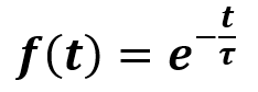
Where e is the Euler number, t is time and τ is the time constant. This funtion produces a time response like this:
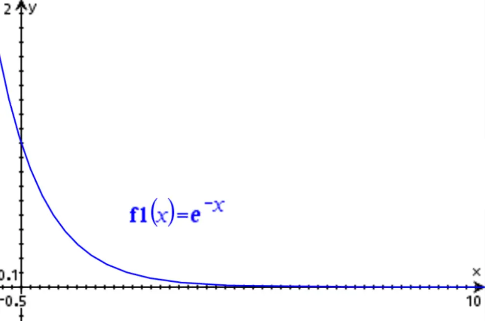
First-order systems exhibit an interesting property: they decay to zero after a time period equal to 5τ has elapsed. For example, if τ=1 (as in the image above), the value of the function will have decayed to 0.67% of its initial value (e-5=0.673), which can be considered effectively extinguished.
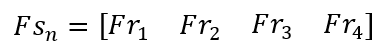
For the Reinforcement Learning algorithm, time is not important, so we focus on episode number. initial_epsilon will be the initial amplitude of the expotential function; final_epsilon is the final value; epsilon_decay is equivalent to τ and random_exp is like a episode delay for the exponential function. We can model this as follows:
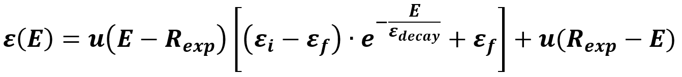
In this function:
- E is the number of the actual episode being played
- ε is the value of the Epsilon function
- Rexp is the number of episodes that will be used for the exploration stage of the algorithm
- εi is the desired initial value of the Epsilon function at the start of Annealing stage
- εf is the desired final value of the Epsilon function at the end of Annealing stage
- εdecay is used to control the speed of the Annealing
- u(E) is a step funtion to represent the two stages of the function
The following chart shows a graphical representation of the Epsilon function:
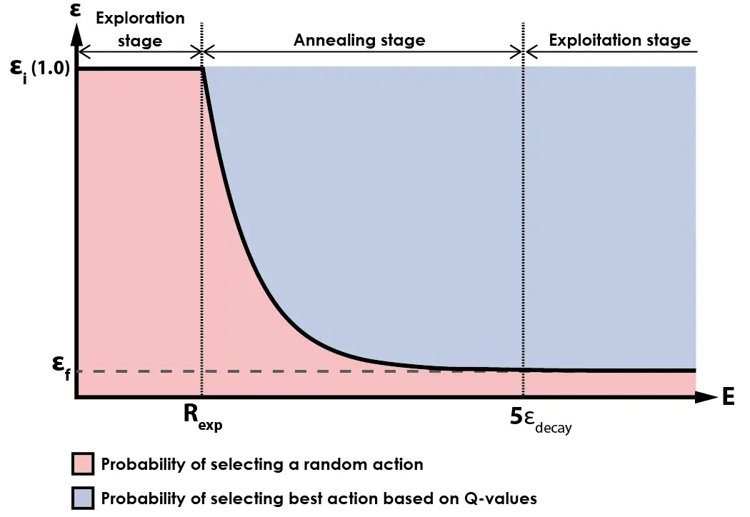
During the initial stage of training, the agent selects actions randomly with a 100% probability. Once the agent has played more than random_exp episodes, the annealing process begins, and the agent starts selecting actions based on its past experience instead of choosing actions randomly.
As the number of episodes played surpasses 5 times the value of epsilon_decay, the algorithm enters its final stage, in which most actions are selected based on the output of the neural network, with a small percentage of actions still selected randomly. This encourages continued exploration of the environment during later stages of training, while also ensuring that the agent mostly selects actions based on what it has learned from experience.
During the development of this algorithm, I have been using a value of 0.05 for the final value of epsilon (εf). This means that after the annealing process is complete, actions will be selected with a 5% probability based on random exploration, and with a 95% probability based on the Q-values learned by the network.
The dqn.py script also features a ReplayMemory Class, with the following code:
|
1 2 3 4 5 6 7 8 9 10 11 12 13 14 15 16 17 18 19 20 21 22 23 24 25 26 27 28 29 30 31 32 33 34 35 36 37 38 39 40 41 |
# Define the replay memory data structure for storing experience tuples class ReplayMemory(object): def __init__(self, capacity, state_shape, device): replay_buffer_capacity,height,width = state_shape # Store the capacity of the memory buffer, the device, and initialize the memory buffer self.capacity = capacity self.device = device self.actions = torch.zeros((capacity, 1), dtype=torch.long) self.states = torch.zeros((capacity, replay_buffer_capacity, height, width), dtype=torch.uint8) self.rewards = torch.zeros((capacity, 1), dtype=torch.int8) self.dones = torch.zeros((capacity, 1), dtype=torch.bool) # Initialize the position and size of the memory buffer self.position = 0 self.size = 0 # Add a new experience tuple to the memory buffer def push(self, state, action, reward, done): self.states[self.position] = state self.actions[self.position,0] = action self.rewards[self.position,0] = reward self.dones[self.position,0] = done # Update the position and size of the memory buffer self.position = (self.position + 1) % self.capacity self.size = max(self.size, self.position) # Sample a batch of experiences from the memory buffer def sample(self, batch_state): i = torch.randint(0, high=self.size, size=(batch_state,)) # Get the current state and next state batch_next_state = self.states[i, 1:] batch_state = self.states[i, :4] # Get the action, reward, and done values for each experience tuple in the batch batch_reward = self.rewards[i].to(self.device).float() batch_done = self.dones[i].to(self.device).float() batch_actions = self.actions[i].to(self.device) # Return the batch of experiences return batch_state, batch_actions, batch_reward, batch_next_state, batch_done # Return the current size of the memory buffer def __len__(self): return self.size |
This class represents a data structure for storing experience tuples in the form (state, action, reward, done, next_state) used in reinforcement learning algorithms.
When initialized, the class takes three parameters:
- capacity: determines the maximum number of tuples that the memory can store
- state_shape: describes the shape of the state tensor
- device: indicates whether to use a GPU or CPU for computations.
The __init__ method initializes the memory buffer with empty tensors to store the tuples. The push method adds a new tuple to the memory buffer at the current position, and updates the position and size of the buffer accordingly.
The sample method returns a batch of batch_state experience tuples randomly sampled from the memory buffer. It retrieves the current state, next state, action, reward, and done values for each tuple in the batch, and returns them as tensors.
The __len__ method returns the current size of the memory buffer.
Replay Memory is a critical component of reinforcement learning algorithms, especially deep Q-learning networks. The purpose of the replay memory is to store past experiences (state, action, reward, next state) and randomly sample a batch of them to train the neural network. This helps the network to learn from a diverse set of experiences, preventing it from overfitting to a specific set of experiences, leading to better generalization to unseen situations.
Replay memory also allows for the breaking of the sequential correlation between experiences, which can cause issues when training the network. By randomly sampling experiences from the memory buffer, the network is exposed to a more diverse set of experiences, and it learns to generalize better.
All these components are packed in the dqn.py script, which is used by agent_trainer.py to train the Reinforcement Learning algorithm to play this game. Let’s move on to the other scripts.
Atari Wrappers
This code is a Python script that contains a set of wrappers for modifying the behavior of Atari environments in OpenAI Gym. These wrappers preprocess raw game screen frames and provide additional features for training reinforcement learning models.
I did not author this code. It is largely based on an OpenAI baseline that can be accessed here, with only minor modifications.
Here’s a brief description of each method in the code, from my understanding:
- NoopResetEnv: This wrapper adds a random number of “no-op” (no-operation) actions to the start of each episode to introduce some randomness and make the agent explore more.
- FireResetEnv: This wrapper automatically presses the “FIRE” button at the start of each episode, which is required for some Atari games to start.
- EpisodicLifeEnv: This wrapper resets the environment whenever the agent loses a life, rather than when the game is over, to make the agent learn to survive for longer periods.
- MaxAndSkipEnv: This wrapper skips a fixed number of frames (usually 4) and returns the maximum pixel value from the skipped frames, to reduce the impact of visual artifacts and make the agent learn to track moving objects.
- ClipRewardEnv: This wrapper clips the reward signal to be either -1, 0, or 1, to make the agent focus on the long-term goal of winning the game rather than short-term rewards.
- WarpFrame: This wrapper resizes and converts the game screen frames to grayscale to reduce the input size and make it easier for the agent to learn.
- FrameStack: This wrapper stacks a fixed number of frames (usually 4) together to give the agent some temporal information and make it easier for the agent to learn the dynamics of the game.
- ScaledFloatFrame: This wrapper scales the pixel values to be between 0 and 1 to make the input data more compatible with deep learning models.
- make_atari: This function creates an Atari environment with various settings suitable for deep reinforcement learning research, including the use of the NoFrameskip wrapper and a maximum number of steps per episode.
- wrap_deepmind: This function applies a combination of the defined wrappers to the given env object, including EpisodicLifeEnv, FireResetEnv, WarpFrame, ClipRewardEnv, and FrameStack. The scale argument can be used to include the ScaledFloatFrame wrapper as well.
From this code only make_atari and wrap_deepmind are used in the agent_trainer.py script, which we are going to describe in the next section.
Agent Trainer
The agent_trainer.py script contains the main training loop for a reinforcement learning agent using the Deep Q-Network (DQN) algorithm. The script initializes the DQN model, sets hyperparameters and creates a replay memory buffer for storing experience tuples.
The script then runs the main training loop for a specified number of episodes, during which the agent interacts with the environment, samples experience tuples from the replay memory buffer, and updates the parameters of the DQN model. The script also periodically evaluates the performance of the agent on a set of evaluation episodes and saves the current DQN model and replay memory buffer to disk for later use.
Now I will go on details with this code. First I want to describe the hyperparameters of the code:
|
1 2 3 4 5 6 7 8 9 10 11 12 13 14 15 16 17 18 |
batch_size = 32 # Number of experiences to sample from the replay buffer for each training iteration gamma = 0.99 # Discount factor used in the Q-learning update equation initial_epsilon = 0.05 # Initial value of the exploration rate for epsilon-greedy action selection strategy final_epsilon = 0.05 # Final value of the exploration rate for epsilon-greedy action selection strategy epsilon_decay = 20000 # Number of steps over which to decay the exploration rate from initial to final value optimizer_epsilon = 1.5e-4 # Learning rate for the optimizer used to update the policy network adam_learning_rate = 0.0000625 # Learning rate for the Adam optimizer used to update the target network target_network_update = 10000 # Frequency (in steps) at which to update the target network episodes = 1000000 # Total number of episodes to train for memory_size = 1000000 # Maximum size of the replay buffer policy_network_update = 4 # Frequency (in steps) at which to update the policy network policy_saving_frequency = 4 # Frequency (in episodes) at which to save the policy network num_eval_episode = 15 # Number of episodes to evaluate the policy network on during evaluation random_exploration_interval = 50000 # Number of steps during which to perform random exploration before using the policy network evaluation_frequency = 50000 # Frequency (in steps) at which to evaluate the policy network max_episode_steps = 40000 # Maximum number of steps to take in each episode frame_stack_size = 4 # Number of frames to stack together to form an input to the neural network previous_experience = 100000 # Number of experiences to collect in the replay buffer before starting training |
By changing these values you can greatly affect the performance of the training algorithm. There are some values that shouldn’t be changes, as they are pretty much standard for this task. That is the case of batch_size, gamma, optimizer_epsilon, adam_learning_rate, target_network_update, memory_size, policy_network_update, policy_saving_frequency, num_eval_episode and frame_stack_size.
Yes, you can try to change those values, but I wouldn’t recommend it until you have a full understanding of the algorithm and how every one of those parameters are used.
The number of episodes is the most significant parameter at the beginning, as it tells the trainer how many episodes to play. To test this algorithm, it is advisable to set the number of episodes to at least 1,000,000, which has been observed to produce human-like scores of around ~35 points. That’s from my experience with this algorithm, with no annealing and with the parameters posted above.
If you set both initial_epsilon and final_epsilon to 0.05, you essentially remove the annealing process from this algorithm. The benefits of annealing can be discussed in a future post, but for now, not using annealing is still effective.
The following chart presents the average reward obtained by an agent with the settings above:
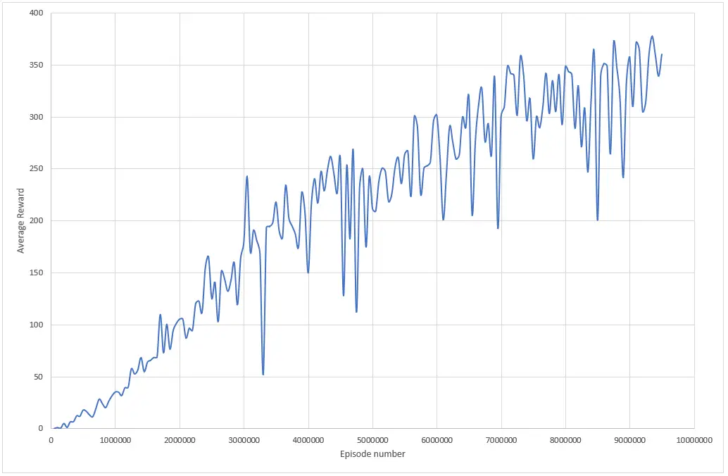
To train an agent that achieves a score greater than 350 points in Breakout, you need to train the agent for at least 9 million episodes using the given parameters. The time required to train the model depends on your hardware resources, with a good GPU being faster than a good CPU. For example, the training process that generated the chart above played 10 million episodes in over 48 hours. However, the same algorithm would complete in 10 hours on an RTX 3060, 6GB GPU. That’s a big gap right there.
The training of an agent can be done on multiple stages, because this script has a mechanism to “save” the training of a model into a new_policy_network.pt file. If you want to use this mechanism, you can train a model with a certain number of episodes and save the training into a file. Then, you rename that file to trained_policy_network.pt and it will load the policy and avoid starting from a blank slate.
This is done by this function:
|
1 2 3 4 5 6 7 8 9 10 11 12 |
def load_pretrained_model(model): # Check if a pre-trained model exists at the specified path if os.path.isfile(pretrained_policy_path): # If a pre-trained model exists, load its state dictionary into the input model print("Loading pre-trained model from", pretrained_policy_path) model.load_state_dict(torch.load(pretrained_policy_path)) else: # If a pre-trained model does not exist, initialize the input model's weights from scratch print("Pre-trained model not found. Training from scratch.") model.apply(model.init_weights) # Return the input model (either loaded with a pre-trained model or initialized from scratch) return model |
That structure makes it easier to train a model on multiple stages. It should be noted that previous_experience provides context to the algorithm, so it will not go through the exploration stage every time experience is added to the policy file.
This script also features the optimize function:
|
1 2 3 4 5 6 7 8 9 10 11 12 13 14 15 16 17 18 19 20 21 22 23 24 |
def optimize_model(train, optimizer, memory, policy_net, target_net): # If the train flag is False, return from the function without optimizing the model if not train: return # Sample a batch of experiences from memory state_batch, action_batch, reward_batch, n_state_batch, done_batch = memory.sample(batch_size) # Compute the Q-values for the current state and action using the policy network q_network = policy_net(state_batch).gather(1, action_batch) # Compute the maximum Q-value for the next state using the target network t_network = target_net(n_state_batch).max(1)[0].detach() # Compute the expected Q-value for the current state and action using the Bellman equation expected_state_action_values = (t_network * gamma) * (1. - done_batch[:, 0]) + reward_batch[:, 0] # Compute the loss between the Q-values predicted by the policy network and the expected Q-values loss = F.smooth_l1_loss(q_network, expected_state_action_values.unsqueeze(1)) # Zero out the gradients of the optimizer optimizer.zero_grad() # Backpropagate the loss through the model loss.backward() # Clip the gradients to be between -1 and 1 for param in policy_net.parameters(): param.grad.data.clamp_(-1, 1) # Update the parameters of the model using the optimizer optimizer.step() |
This is where magic takes place, the actual learning. The train flag is used to determine whether to optimize the model or not. If train is False, the function returns without optimizing the model. That is the exploration stage described in the previous section, which depends on the value of random_exploration_interval hyperparameter.
When train flag is True, a batch of experiences is sampled from memory, and the Q-values for the current state and action are computed using the policy network. The maximum Q-value for the next state is computed using the target network, and the expected Q-value for the current state and action is computed using the Bellman equation.
The loss between the Q-values predicted by the policy network and the expected Q-values is computed using the smooth L1 loss function. The gradients of the optimizer are zeroed out, and the loss is backpropagated through the model. The gradients are then clipped to be between -1 and 1, and the parameters of the model are updated using the optimizer.
Summing it up, the optimize_model function optimizes the PyTorch neural network model by computing and updating the Q-values, expected Q-values, and loss using a batch of experiences stored in memory.
The other important function of this code is evaluate:
|
1 2 3 4 5 6 7 8 9 10 11 12 13 14 15 16 17 18 19 20 21 22 23 24 25 26 27 28 29 30 31 32 33 34 35 36 37 38 39 40 41 42 43 44 45 46 47 48 49 50 51 |
# This function evaluates a PyTorch neural network model on a wrapped OpenAI gym environment def evaluate(step, policy_net, device, env, n_actions, train): # Wrap the OpenAI gym environment in a deepmind wrapper env = wrap_deepmind(env) # Initialize an action selector using hyperparameters and the input policy network action_selector = m.ActionSelector(initial_epsilon, final_epsilon, epsilon_decay, random_exploration_interval, policy_net, n_actions, device) # Initialize an empty list to store the total rewards obtained in each episode total_rewards = [] # Initialize a deque to store a sequence of frames (used for state representation) frame_stack = deque(maxlen=frame_stack_size) # Run a fixed number of evaluation episodes on the environment for i in range(num_eval_episode): # Reset the environment and initialize the episode reward env.reset() episode_reward = 0 # Initialize the frame stack with a sequence of initial frames for _ in range(10): pixels, _, done, _ = env.step(0) pixels = m.fp(pixels) frame_stack.append(pixels) # Loop until the end of the episode is reached while not done: # Concatenate the current frame stack to create the current state representation state = torch.cat(list(frame_stack))[1:].unsqueeze(0) # Select an action using the action selector action, eps = action_selector.select_action(state, step, train) # Take a step in the environment with the selected action and update the frame stack pixels, reward, done, info = env.step(action) pixels = m.fp(pixels) frame_stack.append(pixels) # Update the episode reward episode_reward += reward # Store the episode reward in the total_rewards list total_rewards.append(episode_reward) # Write the average episode reward, current step, and current epsilon to a score record file f = open("score_record.txt", 'a') f.write("%f, %d, %f\n" % (float(sum(total_rewards)) / float(num_eval_episode), step, eps)) f.close() |
This code is for evaluating how well an artificial intelligence agent can perform in a video game environment. The agent uses a neural network to make decisions, and this code helps us understand how good those decisions are.
The code takes the agent’s neural network and runs it on the game environment, which is set up to make it easy for the agent to learn. The code also keeps track of how well the agent is doing by keeping track of the total points it scores in each episode.
After running the agent on the game environment for a set number of episodes, the code calculates the average score across all the episodes and writes it down in a file along with other information, such as the current step and the current level of exploration. This information helps us see how the agent’s performance is improving over time.
This function stores the average episode reward, current step number, and level of exploration in a text file, which helps track the agent’s performance over time.
Finally, it is the Main function that makes all components to work:
|
1 2 3 4 5 6 7 8 9 10 11 12 13 14 15 16 17 18 19 20 21 22 23 24 25 26 27 28 29 30 31 32 33 34 35 36 37 38 39 40 41 42 43 44 45 46 47 48 49 50 51 52 53 54 55 56 57 58 59 60 61 62 63 64 65 66 67 68 69 70 71 72 73 74 75 76 77 78 79 80 81 82 83 84 85 86 87 88 89 90 |
def main(): # Set the CUDA_VISIBLE_DEVICES environment variable to use GPU if available os.environ['CUDA_VISIBLE_DEVICES'] = '0' # Set the device to CUDA if available, else CPU device = torch.device("cuda" if torch.cuda.is_available() else "cpu") # Set the name of the game environment env_name = 'Breakout' # Create a raw Atari environment without frame skipping env_raw = make_atari('{}NoFrameskip-v4'.format(env_name), max_episode_steps, False) # Wrap the Atari environment in a DeepMind wrapper env = wrap_deepmind(env_raw, frame_stack=False, episode_life=True, clip_rewards=True) # Get the replay buffer capacity, height, and width from the first frame replay_buffer_capacity, height, width = m.fp(env.reset()).shape # Get the number of possible actions in the game possible_actions = env.action_space.n # Initialize the policy and target networks using the DQN class policy_network = m.DQN(possible_actions, device).to(device) target_network = m.DQN(possible_actions, device).to(device) # Load the pre-trained policy network, and synchronize the target network with it policy_network=load_pretrained_model(policy_network) target_network.load_state_dict(policy_network.state_dict()) target_network.eval() # Initialize the optimizer using the Adam algorithm optimizer = optim.Adam(policy_network.parameters(), lr=adam_learning_rate, eps=optimizer_epsilon) # Initialize the replay memory buffer memory = m.ReplayMemory(memory_size, [frame_stack_size, height, width], device) # Initialize the action selector action_selector = m.ActionSelector(initial_epsilon, final_epsilon, epsilon_decay, random_exploration_interval,policy_network, possible_actions, device) # Initialize the frame stack and episode length frame_stack = deque(maxlen=frame_stack_size) done = True episode_len = 0 # Initialize the progress bar for training episodes training_progress_bar = tqdm(range(episodes), total=episodes, ncols=50, leave=False, unit='b') # Loop over the training episodes for step in training_progress_bar: # Reset the environment if the episode is done, and initialize the frame stack and episode length if done: env.reset() episode_len = 0 for i in range(10): pixels, _, _, _ = env.step(0) pixels = m.fp(pixels) frame_stack.append(pixels) # Determine whether the agent is currently training or exploring randomly training_flag = len(memory) > max(random_exploration_interval-previous_experience,0) # Create the current state representation using the frame stack state = torch.cat(list(frame_stack))[1:].unsqueeze(0) # Select an action using the action selector, and take the action in the environment action, eps = action_selector.select_action(state, step+previous_experience, training_flag) pixels, reward, done, info = env.step(action) pixels = m.fp(pixels) frame_stack.append(pixels) # Add the current state, action, reward, and done flag to the replay memory buffer memory.push(torch.cat(list(frame_stack)).unsqueeze(0), action, reward, done) episode_len += 1 # Evaluate the performance of the policy network periodically if step % evaluation_frequency == 0: evaluate(step + previous_experience, policy_network, device, env_raw, possible_actions, training_flag) # Optimize the policy network periodically if step % policy_network_update == 0: optimize_model(training_flag, optimizer, memory, policy_network, target_network) # Synchronize the target network with the policy network periodically if step % target_network_update == 0: target_network.load_state_dict(policy_network.state_dict()) # Save the policy network weights periodically if step % policy_saving_frequency == 0: torch.save(policy_network.state_dict(), new_policy_path) |
This is the point where all components of the algorithm come together and training takes place.
Here is a high-level description of the main function:
- The main() function initializes the game environment, sets up the neural networks, optimizer, and other parameters for training the DQN, and begins the training loop.
- The game environment is first created using the make_atari() function from OpenAI Gym, which returns a raw Atari environment without frame skipping.
- The environment is then wrapped in a DeepMind wrapper using the wrap_deepmind() function to preprocess the observations and actions, clip rewards, and stack frames to create the input to the neural networks.
- The neural networks are defined using the DQN() class, which creates a deep convolutional neural network with a specified number of output nodes corresponding to the number of possible actions in the game.
- The load_pretrained_model() function loads a pre-trained policy network if one is available and synchronizes the target network with the policy network.
- The optimizer is defined using the Adam algorithm with a specified learning rate and epsilon.
- The replay memory buffer is initialized using the ReplayMemory() class, which creates a buffer of fixed size to store previous experiences of the agent in the game.
- The action selector is defined using the ActionSelector() class, which selects actions according to an epsilon-greedy policy.
- The training loop consists of a series of episodes, where each episode consists of a sequence of time steps.
- At each time step, the current state of the game is represented using a frame stack of the previous observations, and the action selector selects an action to take based on the current state and exploration policy.
- The environment is stepped forward using the selected action, and the resulting observation, reward, and done flag are stored in the replay memory buffer.
- Periodically, the performance of the policy network is evaluated using the evaluate() function, the policy network is optimized using the optimize_model() function, the target network is synchronized with the policy network, and the policy network weights are saved to disk.
- The training loop terminates after a fixed number of episodes, and the final policy network weights are saved to disk.
By running this main function the training will start and the agent will learn from the experience. After finishing it, a policy file will be generated, wich can be used for playing the game automatically with a Renderer script.


