
Reinforcement Learning es una rama de la Inteligencia Artificial que se ocupa del desarrollar algoritmos y modelos capaces de aprender a través de retroalimentación y optimizar acciones para lograr un objetivo específico. Una aplicación popular del aprendizaje por refuerzo es entrenar un agente de inteligencia artificial (IA) para jugar videojuegos.
En este post veremos cómo utilizar Reinforcement Learning para entrenar a un agente de IA para jugar al clásico juego de Atari, Breakout. Utilizaremos un algoritmo con una Deep Q-Network (DQN), que es una técnica popular para entrenar agentes de IA que juegan videojuegos.
Este será un tutorial paso a paso sobre cómo implementar el algoritmo DQN en Python utilizando PyTorch y el entorno OpenAI Gym para entrenar a un agente de IA para jugar Atari Breakout.
El resultado del entrenamiento de un agente con 20 millones de episodios de experiencia lo pueden ver en el siguiente video:
Al final de este post habremos explicado los principales componentes de este algoritmos, junto con detalles sobre su funcionamiento y los scripts utilizados para lograr estos resultados. Sin más que decir, comencemos.
Qué es Reinforcement Learning?
Reinforcement Learning (aprendizaje por reforzamiento) es un subcampo de la inteligencia artificial (IA) que se enfoca en desarrollar algoritmos y modelos que permiten a los agentes aprender a través de la retroalimentación para optimizar sus acciones y lograr un objetivo particular.
En Reinforcement Learning un agente interactúa con un entorno y recibe recompensas o penalizaciones por sus acciones. Luego, el agente utiliza esta retroalimentación para actualizar su proceso de toma de decisiones y mejorar sus acciones futuras para maximizar la recompensa acumulada con el tiempo.
RL ha sido aplicado exitosamente en diversos campos, como la robótica, los juegos, los sistemas de recomendación y más. La principal ventaja del aprendizaje por refuerzo es su habilidad para aprender mediante ensayo y error sin requerir un conjunto predefinido de reglas o ejemplos.
No tengo la intención de explorar este tema más a fondo en esta publicación, ya que planeo escribir un post dedicado a explicar en detalle el concepto de Reinforcement Learning.
En este post lo que haré será utiizar algoritmos de RL para entrenar a un agente de IA para jugar Atari Breakout. Para lograr esto, crearemos un entorno donde el agente pueda jugar el juego, tomar decisiones y aprender de los resultados de esas decisiones. Después de varias horas de entrenamiento, el agente debería ser capaz de jugar el juego a un alto nivel por sí solo.
Antes de empezar con el código
El código con el algoritmo que describiremos en este post lo pueden descargar directamente desde nuestro repositorio de Github.
Si usted quiere replicar los resultados obtenidos en el video mostrado en la parte superior, esto lo podrpa hacer descargando el repositorio y ejecutando el archivo renderer.py. Este archivo utilizará el policy que hemos compartido en el repositorio, el cual cuenta con 20 millones de episodios de experiencia.
Para ejecutar este código se necesita instalar Pytorch, algo que ya explicamos en este post. No será necesario instalar OpenAI Gym, pues la biblioteca ha sido incluida en el repositorio en el directorio gym. Se decidió hacer esto de esta manera pues el algoritmo nos estaba dando problemas con la versión más reciente del Gym, por lo cual agregamos una versión modificada en la que se han corregido los errores que se producían al ejecutar el algoritmo con la versión 0.26.2.
También hará falta instalar Numpy y algunas otras dependencias, pero eso no debe ser un problema para cualquier persona con un mínimo de conocimiento en Python.
Composición del algoritmo
La siguiente imagen presenta una representación visual de los scripts que conforman este proyecto:
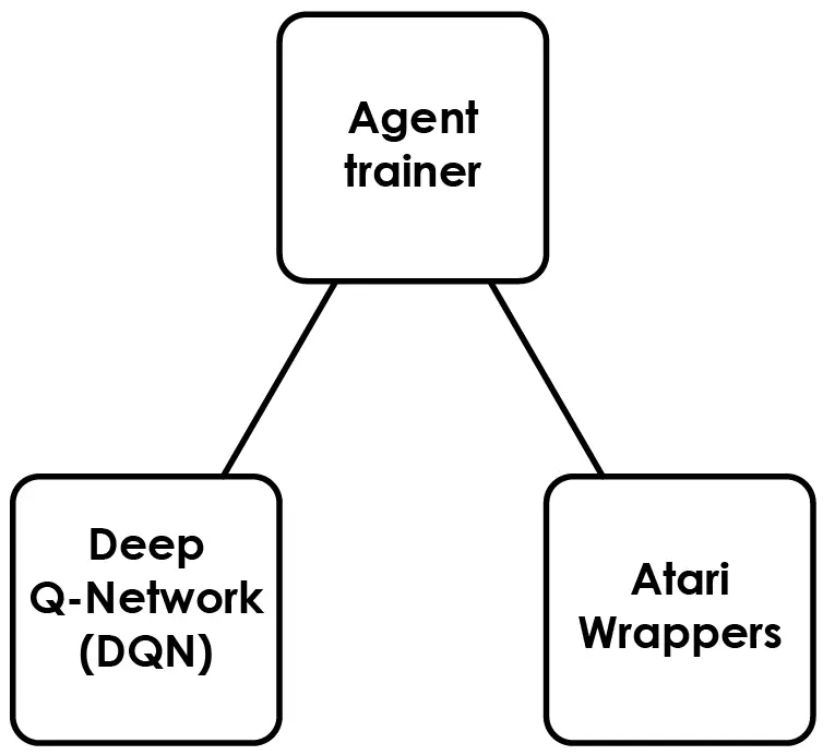
Cada componente ha sido construido como un script separado de Python, los cuales se pueden encontrar en nuestro repositorio de Github. Aquí hay una descripción de alto nivel de cada componente:
- Deep Q-Network (DNQ): un script de Python que define la arquitectura de la red neuronal, la estrategia de selección de acciones epsilon-greedy, el búfer de memoria de replays y una función para convertir los cuadros de imagen (capturas de pantalla) de entrada en tensores PyTorch para el algoritmo de Deep Q-Network (DQN).
- Agent trainer: script en Python que entrena una red neuronal para aprender cómo jugar el juego utilizando el Reinforcement Learning y guarda el policy de red entrenada en un archivo.
- Atari Wrappers: un script en Python que contiene un conjunto de funciones (wrappers) que permiten interactuar con el juego de Atari. Este script permite ejecutar acciones en el juego, tales como mover el pad de izquierda a derecha. Tambien permite conocer el puntaje del juego y el estado del juego (una captura de pantalla).
Este proyecto también incluye el script de renderizado (el previamente mencionado renderer.py), que carga un archivo policy con el entrenamiento y lo utiliza para jugar el juego. Esto nos permite observar el progreso del agente visualmente y evaluar su rendimiento en tiempo real.
A continuación proporcionaré una explicación detallada de cada script, lo que le permitirá obtener una mejor comprensión del funcionamiento interno de este algoritmo.
Deep Q-Network (DNQ)
Esta parte del algoritmo ha sido construida en el script dqn.py. Define la arquitectura de la red neuronal para el algoritmo de Deep Q-Network (DQN), que se utiliza para entrenar a un agente para jugar un juego a partir de entrada de píxeles. Estio se hizo utilizando Pytorch.
La arquitectura de la red neuronal consta de capas convolucionales seguidas de capas completamente conectadas. El agente aprende a jugar el juego utilizando el aprendizaje por refuerzo interactuando con el entorno y actualizando los pesos de la red neuronal en consecuencia.
A continuación les traemos la representación gráfica de la red neuronal:
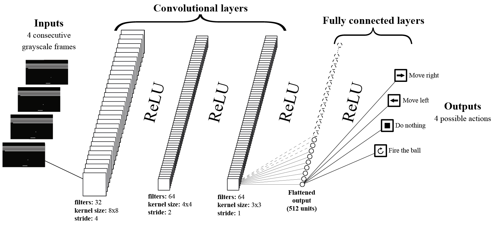
Esta arquitectura de red neuronal toma como entrada 4 frames (capturas de patalla) consecutivos. Cada frame se representa como una matriz 3D de píxeles, que se puede obtener utilizando el Atari Wrappers. Luego, los frames se convierten a escala de grises, reduciendo efectivamente las 3 dimensiones de color a una sola, lo que resulta en una representación de matriz 2D.
Este proceso lo hemos representado en la siguiente imagen:
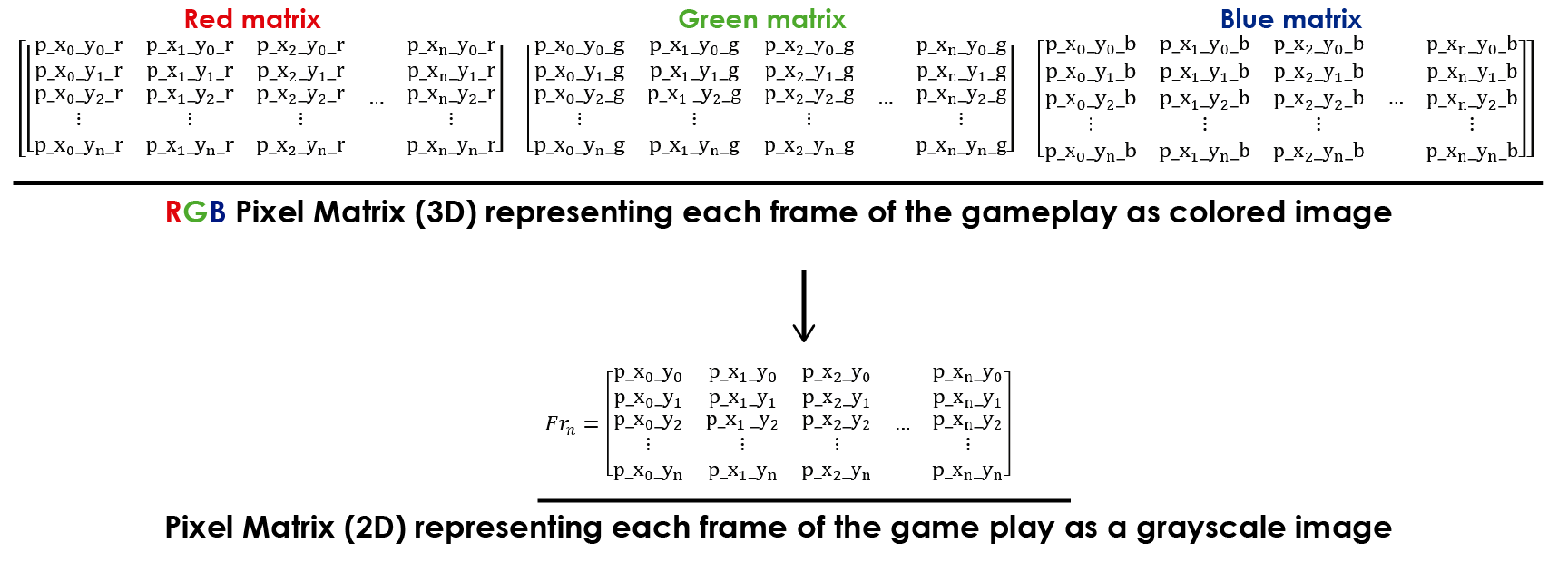
Reducir las dimensiones de la entrada es ventajoso para entrenar la red neuronal ya que reduce la cantidad de información que se debe procesar. En este juego, el color no es crucial para reconocer características significativas que podrían ayudar al aprendizaje del del entorno.
En el script la reducción de dimensión se lleva a cabo en la siguiente función:
|
1 2 3 4 |
def get_frame_tensor(pixels): pixels = torch.from_numpy(pixels) height = pixels.shape[-2] return pixels.view(1, height, height) |
Estas líneas de código transforman las dimensiones de la imagen de 3 a 1 y redimensionan la imagen en una forma cuadrada (altura por altura). Esto comprime la imagen y reduce su tamaño, lo que conduce a una pérdida menor de datos. Sin embargo, esta transformación simplifica el procesamiento de la imagen.
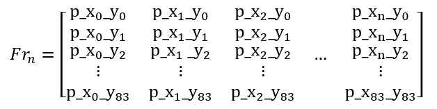
Dicho esto, cada frame se representará como una matriz como esta:
Al usar 4 frames consecutivos del juego como entrada, podemos proporcionar una mejor información sobre lo que está sucediendo en el juego. Un solo cuadro no muestra suficiente contexto, como si la pelota se mueve hacia arriba o hacia abajo o qué tan rápido se está moviendo.
Estos 4 frames son empacados en una nueva matrix, la Frame Stack Matrix:
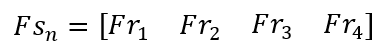
La Frame Stack Matrix puede parecer una matriz 2D, pero en realidad es una matriz 3D. Cada índice en la matriz contiene un frame, que es una matriz 2D.
Finalmente, combinaremos 32 Frame Stack Matrix en un «batch» que es una matriz 4D. Esta matriz 4D, también conocida como input tensor, se pasará como entrada a la red neuronal.

Al entrenar la red neuronal, cada elemento del tensor de entrada se pasará a través de la red neuronal, como se muestra en la representación gráfica de la Red Neuronal de Aprendizaje Profundo de Q (ver arriba).
La estructura de la red neuronal se define en el constructor de la clase DQN:
|
1 2 3 4 5 6 7 8 9 10 11 12 |
class DQN(nn.Module): def __init__(self, outputs, device): super(DQN, self).__init__() # Define the convolutional layers self.conv1 = nn.Conv2d(4, 32, kernel_size=8, stride=4, bias=False) self.conv2 = nn.Conv2d(32, 64, kernel_size=4, stride=2, bias=False) self.conv3 = nn.Conv2d(64, 64, kernel_size=3, stride=1, bias=False) # Define the fully connected layers self.fc1 = nn.Linear(64 * 7 * 7, 512) self.fc2 = nn.Linear(512, outputs) # Store the device where the model will be trained self.device = device |
Este código de la Red Neuronal en PyTorch es relativamente fácil de entender, con una conexión clara entre el código y su representación gráfica.
Durante el entrenamiento de esta red, se utiliza la función «forward»:
|
1 2 3 4 5 6 7 8 |
# Define the forward pass of the neural network def forward(self, x): x = x.to(self.device).float() / 255. x = F.relu(self.conv1(x)) x = F.relu(self.conv2(x)) x = F.relu(self.conv3(x)) x = F.relu(self.fc1(x.view(x.size(0), -1))) return self.fc2(x) |
Esta función toma el tensor de entrada «x» y calcula los valores Q para las cuatro acciones que el agente puede elegir, basándose en los cuatro fotogramas anteriores del juego.
Las 4 posibles acciones son:
-
- Mover el paddle hacia la izquierda
- Mover el paddle hacia la derecha
- No hacer nada (es decir, mantenerse en la misma posición)
- Disparar la pelota (no es una acción comúnmente utilizada)
En este contexto, los Q-values representan la recompensa futura esperada que un agente recibirá si realiza una determinada acción en un estado dado. En el caso del juego Atari Breakout, los Q-values calculados por esta función representan la recompensa futura esperada para cada una de las cuatro posibles acciones, basándose en el estado actual del juego observado a través de los cuatro fotogramas anteriores. El agente utiliza estos Q-values para determinar qué acción tomar con el fin de maximizar su recompensa acumulada a lo largo del tiempo.
Al comienzo del entrenamiento, el agente no tiene experiencia en el entorno y no puede predecir la ganancia que obtendrá luego de cada acción. Por lo tanto, la red neuronal no puede producir Q-values apropiados. Sin embargo, después de jugar el juego varias veces, la red neuronal aprenderá a predecir la recompensa futura de tomar una determinada acción basada en el estado del juego (tensor de entrada).
Este script contiene una función para inicializar los pesos de la red neuronal al inicio del entrenamiento:
|
1 2 3 4 5 6 7 |
# Initialize the weights of the neural network def init_weights(self, m): if type(m) == nn.Linear: torch.nn.init.kaiming_normal_(m.weight, nonlinearity='relu') m.bias.data.fill_(0.0) if type(m) == nn.Conv2d: torch.nn.init.kaiming_normal_(m.weight, nonlinearity='relu') |
Esto crea una un estado inicial sin experiencia previa, lo que permite que el agente aprenda de su entorno adquiriendo experiencia mientras juega el juego.
Exploación vs. Explotación
El algoritmo DQN utiliza una combinación de explotación y exploración para aprender del entorno. Durante las etapas iniciales del entrenamiento, el agente necesita explorar el entorno para aprender sobre las acciones disponibles y sus efectos. Para lograr esto, el algoritmo utiliza una variable llamada random_exploration_interval, que determina la cantidad de episodios que el agente debe explorar antes de cambiar a la explotación. Exploración significa realizar movimientos aleatorios para ver qué sucede.
Si el número de episodios jugados es menor que random_exploration_interval, el agente seleccionará acciones al azar para explorar el entorno. Esto fomenta que el agente tome riesgos y pruebe nuevas acciones, incluso si no se han intentado antes. En esta etapa, se calculan los Q-values, pero no se consideran para la selección de acciones.
Una vez que el agente ha jugado suficientes episodios para superar el límite establecido con random_exploration_interval, el comportamiento cambiará a la explotación y se empezará a tomar acciones basadas en los Q-values aprendidos por la red neuronal. Sin embargo, para asegurarse de que el agente continúe explorando el entorno y evite quedar atrapado en óptimos locales, el algoritmo utiliza una técnica llamada epsilon decay o annealing. Esto disminuye gradualmente la probabilidad de seleccionar una acción aleatoria con el tiempo, de modo que el agente se vuelve cada vez más propenso a seleccionar acciones basadas en los Q-values a medida que adquiere experiencia.
Todo este proceso ha sido codificado en la clase ActionSelector:
|
1 2 3 4 5 6 7 8 9 10 11 12 13 14 15 16 17 18 19 20 21 22 23 24 |
class ActionSelector(object): def __init__(self, initial_eps, final_eps, eps_decay,random_exp, policy_net, n_actions, dev): self.eps = initial_eps self.final_epsilon = final_eps self.initial_epsilon = initial_eps self.random_exploration_interval = random_exp self.policy_network = policy_net self.epsilon_decay = eps_decay self.possible_actions = n_actions self.device = dev def select_action(self, state, current_episode, training=False): sample = random.random() if training: # Update the value of epsilon during training based on the current episode self.eps = self.final_epsilon + (self.initial_epsilon - self.final_epsilon) * \ math.exp(-1. * (current_episode-self.random_exploration_interval) / self.epsilon_decay) self.eps = max(self.eps, self.final_epsilon) if sample > self.eps: with torch.no_grad(): a = self.policy_network(state).max(1)[1].cpu().view(1, 1) else: a = torch.tensor([[random.randrange(self.possible_actions)]], device=self.device, dtype=torch.long) return a.cpu().numpy()[0, 0].item(), self.eps |
El constructor toma los siguientes parámetros como entradas:
- initial_epsilon
- final_epsilon
- epsilon_decay
- random_exp
Estos parámetros se utilizan para modelar la función de decaimiento (Annealing), que exhibe un comportamiento consistente con la respuesta de un sistema de primer orden, similar a un circuito de descarga RL o RC. La descarga de un sistema de primer orden se puede modelar de la siguiente manera:
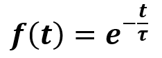
Donde e es el número de Euler, t es el tiempo y τ es la constante de tiempo. Esta función produce una respuesta en el tiempo como esta:
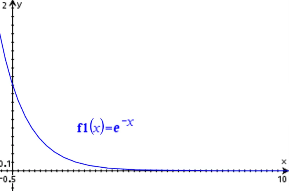
Los sistemas de primer orden presentan una propiedad interesante: se desvanecen a cero después de que haya transcurrido un período de tiempo igual a 5τ. Por ejemplo, si τ = 1 (como en la imagen de arriba), el valor de la función se habrá desvanecido al 0.67% de su valor inicial (e-5 = 0.673), lo que se puede considerar efectivamente extinto.
Para el algoritmo de Reinforcement Learning, el tiempo no es relevante, por lo que nos enfocamos en el número de episodios jugados. initial_epsilon será la amplitud inicial de la función exponencial, final_epsilon es el valor final, epsilon_decay es equivalente a τ y random_exp es como un retraso de episodio para la función exponencial. Podemos modelar esto de la siguiente manera:
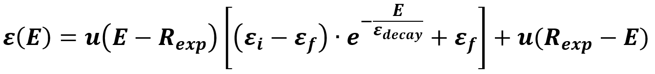
En esta funcion:
- E is the número del episodio actual que se está jugando
- ε es el valor de la función Epsilon
- Rexp es el número de episodios que se utilizarán para la etapa de exploración del algoritmo
- εi es el valor inicial deseado de la función Epsilon al comienzo de la etapa de Annealing
- εf es el valor final deseado de la función Epsilon al final de la etapa de Annealing
- εdecay se utiliza para controlar la velocidad del Annealing
- u(E) es una función escalón para representar las dos etapas de la función
La siguiente gráfica muestra una representación gráfica de la función Epsilon:
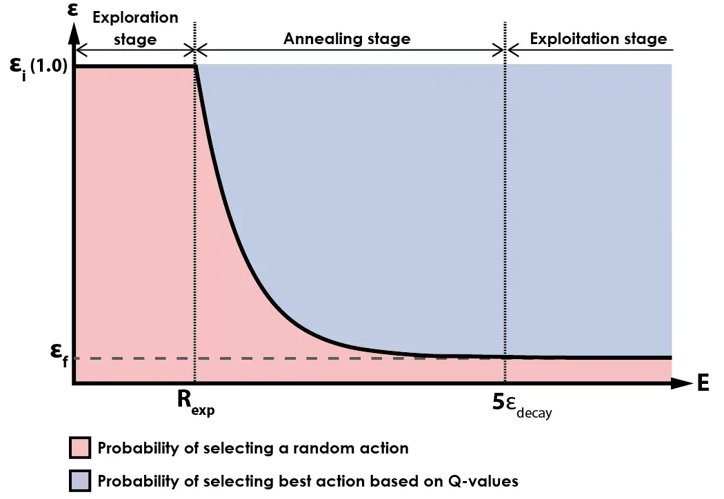
Durante la etapa inicial del entrenamiento, el agente selecciona acciones al azar con una probabilidad del 100%. Una vez que el agente ha jugado más de random_exp episodios, comienza el proceso de annealing y el agente comienza a seleccionar acciones basadas en su experiencia previa en lugar de elegir acciones al azar.
A medida que el número de episodios jugados supera 5 veces el valor de epsilon_decay, el algoritmo entra en su etapa final, en la cual la mayoría de las acciones se seleccionan en base a la salida de la red neuronal (Q-vaues), con un pequeño porcentaje de acciones aún seleccionadas al azar. Esto fomenta la exploración continua del entorno durante las etapas posteriores del entrenamiento, al tiempo que garantiza que el agente seleccione principalmente acciones basadas en lo que ha aprendido de la experiencia.
Durante el desarrollo de este algoritmo, he estado utilizando un valor de 0.05 para el valor final de epsilon (εf). Esto significa que después de que el proceso de annealing esté completo, las acciones se seleccionarán con una probabilidad del 5% basada en la exploración aleatoria, y con una probabilidad del 95% basada en los Q-values aprendidos por la red.
Replay Memory
El script dqn.py también incluye una clase ReplayMemory, con el siguiente código:
|
1 2 3 4 5 6 7 8 9 10 11 12 13 14 15 16 17 18 19 20 21 22 23 24 25 26 27 28 29 30 31 32 33 34 35 36 37 38 39 40 41 |
# Define the replay memory data structure for storing experience tuples class ReplayMemory(object): def __init__(self, capacity, state_shape, device): replay_buffer_capacity,height,width = state_shape # Store the capacity of the memory buffer, the device, and initialize the memory buffer self.capacity = capacity self.device = device self.actions = torch.zeros((capacity, 1), dtype=torch.long) self.states = torch.zeros((capacity, replay_buffer_capacity, height, width), dtype=torch.uint8) self.rewards = torch.zeros((capacity, 1), dtype=torch.int8) self.dones = torch.zeros((capacity, 1), dtype=torch.bool) # Initialize the position and size of the memory buffer self.position = 0 self.size = 0 # Add a new experience tuple to the memory buffer def push(self, state, action, reward, done): self.states[self.position] = state self.actions[self.position,0] = action self.rewards[self.position,0] = reward self.dones[self.position,0] = done # Update the position and size of the memory buffer self.position = (self.position + 1) % self.capacity self.size = max(self.size, self.position) # Sample a batch of experiences from the memory buffer def sample(self, batch_state): i = torch.randint(0, high=self.size, size=(batch_state,)) # Get the current state and next state batch_next_state = self.states[i, 1:] batch_state = self.states[i, :4] # Get the action, reward, and done values for each experience tuple in the batch batch_reward = self.rewards[i].to(self.device).float() batch_done = self.dones[i].to(self.device).float() batch_actions = self.actions[i].to(self.device) # Return the batch of experiences return batch_state, batch_actions, batch_reward, batch_next_state, batch_done # Return the current size of the memory buffer def __len__(self): return self.size |
Esta clase representa una estructura de datos para almacenar tuplas de experiencia en forma de (state, action, reward, done, next_state) utilizadas en algoritmos de Reinforcement Learning.
Cuando se inicializa, la clase toma tres parámetros:
- capacity: determina el número máximo de tuplas que la memoria puede almacenar
- state_shape: describe la forma del tensor de estado
- device: indica si se utilizará una GPU o CPU para los cálculos.
El método init inicializa el búfer de memoria con tensores vacíos para almacenar las tuplas. El método push agrega una nueva tupla al búfer de memoria en la posición actual y actualiza la posición y el tamaño del búfer en consecuencia.
Antes de seguir debo aclarar que una tupla es una estructura de datos que puede contener múltiples elementos. En el contexto del Reinforcement Learning, una tupla generalmente se refiere a un conjunto de elementos que representan una experiencia de interacción entre el agente y el entorno. En este caso el término hace una referencia a una matriz que contiene state, action, reward, done, next_state.
El método sample devuelve un lote (batch) de tuplas de experiencia (experience tuples) del búfer de memoria, seleccionadas de forma aleatoria. Recupera el estado actual, el estado siguiente, la acción, la recompensa y los valores de finalización (done) para cada tupla en el lote y los devuelve como tensores.
El método len devuelve el tamaño actual del búfer de memoria.
La Replay Memory es un componente crítico de los algoritmos de Reinforcement Learning, especialmente de las redes de Q-learning como la que hemos implementado en este proyecto. El propósito de la memoria de repetición es almacenar experiencias pasadas (state, action, reward, done, next_state) y muestrear aleatoriamente un lote de ellas para entrenar la red neuronal. Esto ayuda a la red a aprender de un conjunto diverso de experiencias, evitando el overfitting y permitiendo una mejor generalización a situaciones no vistas previamente.
La Replay Memory también permite romper la correlación secuencial entre experiencias, lo cual puede causar problemas durante el entrenamiento de la red. Al muestrear experiencias de forma aleatoria desde el búfer de memoria, la red se expone a un conjunto de experiencias más diverso y aprende una mejor generalización.
Todos estos componentes están incluidos en el script dqn.py, que es utilizado por agent_trainer.py para entrenar el algoritmo de Reinforcement Learning para jugar este juego. Sigamos adelante con los otros scripts.
Atari Wrappers
Este código es un script de Python que contiene un conjunto de wrappers para modificar el comportamiento de los entornos Atari en OpenAI Gym. Estos wrappers son funciones que preprocesan los fotogramas de la pantalla del juego y proporcionan características adicionales para entrenar modelos de Reinforcement Learning.
Debo aclarar que yo NO he creado este código. Está basado en gran medida en una línea baseline de OpenAI que se puede acceder aquí, con solo modificaciones menores.
Aquí tienes una breve descripción de cada método en el código, según mi comprensión:
- NoopResetEnv: Este wrapper agrega un número aleatorio de acciones «no-op» (no operación) al comienzo de cada episodio para introducir cierta aleatoriedad y hacer que el agente explore más.
- FireResetEnv: Este wrapper presiona automáticamente el botón «FIRE» al comienzo de cada episodio, lo cual es necesario para que algunos juegos de Atari comiencen.
- EpisodicLifeEnv: Este wrapper reinicia el entorno cada vez que el agente pierde una vida, en lugar de hacerlo cuando el juego termina, para hacer que el agente aprenda a sobrevivir durante períodos más largos.
- MaxAndSkipEnv: Este wrapper omite un número fijo de fotogramas (generalmente 4) y devuelve el valor máximo de píxel de los fotogramas omitidos, para reducir el impacto de los visual artifacts y hacer que el agente aprenda a seguir objetos en movimiento.
- ClipRewardEnv: Este wrapper recorta la señal de recompensa para que sea -1, 0 o 1, para que el agente se centre en el objetivo a largo plazo de ganar el juego en lugar de las recompensas a corto plazo.
- WarpFrame: Este wrapper redimensiona y convierte los fotogramas de la pantalla del juego a escala de grises para reducir el tamaño de entrada y facilitar el aprendizaje del agente.
- FrameStack: Este wrapper apila un número fijo de fotogramas (generalmente 4) juntos para proporcionar al agente información temporal y facilitar el aprendizaje de la dinámica del juego.
- ScaledFloatFrame: Este wrapper escala los valores de píxel para que estén entre 0 y 1, para que los datos de entrada sean más compatibles con los modelos de aprendizaje profundo.
- make_atari: Esta función crea un entorno de Atari con varias configuraciones adecuadas para investigaciones de aprendizaje por refuerzo profundo, incluyendo el uso del wrapper NoFrameskip y un número máximo de pasos por episodio.
- wrap_deepmind: Esta función aplica una combinación de los wrappers definidos al objeto env dado, incluyendo EpisodicLifeEnv, FireResetEnv, WarpFrame, ClipRewardEnv y FrameStack. El argumento de escala se puede usar para incluir también el wrapper ScaledFloatFrame.
De este código, solo se utilizan las funciones make_atari y wrap_deepmind en el script agent_trainer.py, el cual describiremos en la próxima sección.
Agent Trainer
El script agent_trainer.py contiene el loop principal de entrenamiento para un agente de Reinforcement Learning utilizando el algoritmo Deep Q-Network (DQN). El script inicializa el modelo DQN, establece hiperparámetros y crea un búfer de memoria de repetición para almacenar tuplas de experiencia.
Luego, el script ejecuta el loop de entrenamiento durante un número determinado de episodios, durante los cuales el agente interactúa con el entorno, muestrea tuplas de experiencia del Replay Memory y actualiza los parámetros del modelo DQN. El script también evalúa periódicamente el rendimiento del agente en un conjunto de episodios de evaluación y guarda un archivo «policy» con la información del entrenamiento de la red neuronal.
Ahora voy a describir en detalle este código. Primero, quiero describir los hiperparámetros:
|
1 2 3 4 5 6 7 8 9 10 11 12 13 14 15 16 17 18 |
batch_size = 32 # Número de experiencias para muestrear del búfer de repetición en cada iteración de entrenamiento gamma = 0.99 # Factor de descuento utilizado en la ecuación de actualización de Q-learning initial_epsilon = 0.05 # Valor inicial de la tasa de exploración para la estrategia de selección de acciones epsilon-greedy final_epsilon = 0.05 # Valor final de la tasa de exploración para la estrategia de selección de acciones epsilon-greedy epsilon_decay = 20000 # Número de pasos durante los cuales se reduce gradualmente la tasa de exploración desde el valor inicial al final optimizer_epsilon = 1.5e-4 # Tasa de aprendizaje para el optimizador utilizado para actualizar la red de política adam_learning_rate = 0.0000625 # Tasa de aprendizaje para el optimizador Adam utilizado para actualizar la red objetivo target_network_update = 10000 # Frecuencia (en pasos) para actualizar la red objetivo episodes = 1000000 # Número total de episodios para entrenar memory_size = 1000000 # Tamaño máximo del búfer de repetición policy_network_update = 4 # Frecuencia (en pasos) para actualizar la red de política policy_saving_frequency = 4 # Frecuencia (en episodios) para guardar la red de política num_eval_episode = 15 # Número de episodios para evaluar la red de política durante la evaluación random_exploration_interval = 10000 # Número de pasos durante los cuales realizar exploración aleatoria antes de utilizar la red de política evaluation_frequency = 25000 # Frecuencia (en pasos) para evaluar la red de política max_episode_steps = 400000 # Número máximo de pasos para tomar en cada episodio frame_stack_size = 5 # Número de fotogramas para apilar juntos y formar una entrada a la red neuronal previous_experience = 100000 # Número de experiencias para recopilar en el búfer de repetición antes de comenzar el entrenamiento |
Al cambiar estos valores, puedes afectar en gran medida el rendimiento del algoritmo de entrenamiento. Hay algunos valores que no deben cambiarse, ya que son bastante estándar para esta tarea. Ese es el caso de batch_size, gamma, optimizer_epsilon, adam_learning_rate, target_network_update, memory_size, policy_network_update, policy_saving_frequency, num_eval_episode y frame_stack_size.
Sí, puedes intentar cambiar esos valores, pero no lo recomendaría hasta que entiendas completamente el algoritmo y cómo se utilizan cada uno de esos parámetros.
El número de episodios es el parámetro más significativo al principio, ya que le indica al entrenador cuántos episodios jugar. Para probar este algoritmo, se recomienda establecer el número de episodios en al menos 1,000,000, lo cual se ha observado que produce puntuaciones similares a las de los humanos, alrededor de ~35 puntos. Esto es a partir de mi experiencia con este algoritmo, sin annealing y con los parámetros mencionados anteriormente.
Si estableces tanto initial_epsilon como final_epsilon en 0.05, básicamente eliminas el proceso de annealing de este algoritmo. Los beneficios del annealing pueden discutirse en una publicación futura.
La siguiente gráfica presenta el promedio del puntaje obtenido por el agente en función de los episodios jugados, para los primeros 10 millones de episodios.
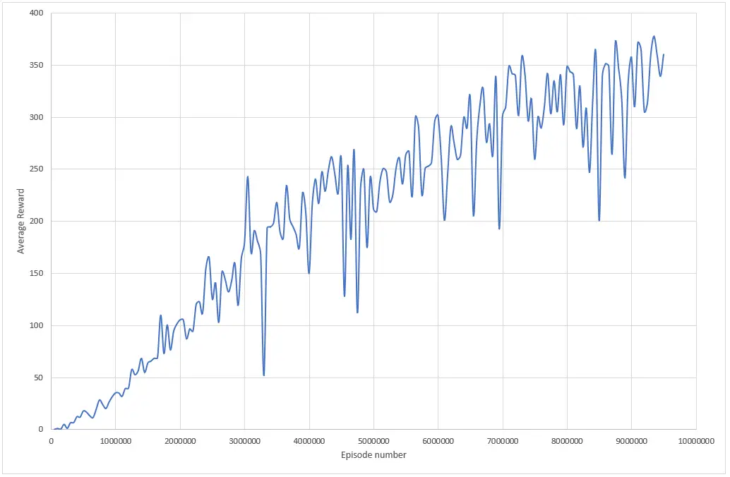
Para entrenar un agente que logre una puntuación superior a 350 puntos en Atari Breakout, necesitas entrenar al agente durante al menos 9 millones de episodios utilizando los parámetros dados. El tiempo requerido para entrenar el modelo depende de los recursos de hardware disponibles, siendo una buena GPU más rápida que una buena CPU.
Por ejemplo, el proceso de entrenamiento que generó el gráfico anterior jugó 10 millones de episodios en más de 48 horas. Sin embargo, el mismo algoritmo se completaría en 10 horas en una GPU RTX 3060 de 6 GB. Esa es una gran diferencia.
El entrenamiento de un agente se puede realizar en varias etapas, ya que este script tiene un mecanismo para «guardar» el entrenamiento de un modelo en un nuevo archivo new_policy_network.pt. Si deseas utilizar este mecanismo, puedes entrenar un modelo con un número determinado de episodios y guardar el entrenamiento en un archivo. Luego, puedes cambiar el nombre de ese archivo a trained_policy_network.pt y se cargará la política y evitará comenzar desde cero.
Esto se realiza mediante esta función:
|
1 2 3 4 5 6 7 8 9 10 11 12 |
def load_pretrained_model(model): # Check if a pre-trained model exists at the specified path if os.path.isfile(pretrained_policy_path): # If a pre-trained model exists, load its state dictionary into the input model print("Loading pre-trained model from", pretrained_policy_path) model.load_state_dict(torch.load(pretrained_policy_path)) else: # If a pre-trained model does not exist, initialize the input model's weights from scratch print("Pre-trained model not found. Training from scratch.") model.apply(model.init_weights) # Return the input model (either loaded with a pre-trained model or initialized from scratch) return model |
Esa estructura facilita el entrenamiento de un modelo en múltiples etapas. Cabe destacar que previous_experience proporciona contexto al algoritmo, por lo que no pasará por la etapa de exploración cada vez que se agregue experiencia al archivo de políticas.
Este script también incluye la función optimize:
|
1 2 3 4 5 6 7 8 9 10 11 12 13 14 15 16 17 18 19 20 21 22 23 24 |
def optimize_model(train, optimizer, memory, policy_net, target_net): # If the train flag is False, return from the function without optimizing the model if not train: return # Sample a batch of experiences from memory state_batch, action_batch, reward_batch, n_state_batch, done_batch = memory.sample(batch_size) # Compute the Q-values for the current state and action using the policy network q_network = policy_net(state_batch).gather(1, action_batch) # Compute the maximum Q-value for the next state using the target network t_network = target_net(n_state_batch).max(1)[0].detach() # Compute the expected Q-value for the current state and action using the Bellman equation expected_state_action_values = (t_network * gamma) * (1. - done_batch[:, 0]) + reward_batch[:, 0] # Compute the loss between the Q-values predicted by the policy network and the expected Q-values loss = F.smooth_l1_loss(q_network, expected_state_action_values.unsqueeze(1)) # Zero out the gradients of the optimizer optimizer.zero_grad() # Backpropagate the loss through the model loss.backward() # Clip the gradients to be between -1 and 1 for param in policy_net.parameters(): param.grad.data.clamp_(-1, 1) # Update the parameters of the model using the optimizer optimizer.step() |
Aquí es donde ocurre la magia, el verdadero aprendizaje. El indicador train se utiliza para determinar si se debe optimizar el modelo o no. Si train es False, la función retorna sin optimizar el modelo. Esa es la etapa de exploración descrita en la sección anterior, que depende del valor del hiperparámetro random_exploration_interval.
Cuando el indicador train es True, se muestrea un lote de experiencias de la memoria, y se calculan los valores Q para el estado y la acción actual utilizando la red de políticas. El valor Q máximo para el siguiente estado se calcula utilizando la red objetivo, y se calcula el valor Q esperado para el estado y la acción actual utilizando la ecuación de Bellman.
La pérdida entre los valores Q predichos por la red de políticas y los valores Q esperados se calcula utilizando la función de pérdida smooth L1. Los gradientes del optimizador se reinician a cero y se realiza la retropropagación de la pérdida a través del modelo. Luego, los gradientes se recortan para que estén entre -1 y 1, y se actualizan los parámetros del modelo utilizando el optimizador.
En resumen, la función optimize_model optimiza el modelo de red neuronal PyTorch calculando y actualizando los valores Q, los valores Q esperados y la pérdida utilizando un lote de experiencias almacenadas en la memoria.
La otra función importante de este código es evaluate:
|
1 2 3 4 5 6 7 8 9 10 11 12 13 14 15 16 17 18 19 20 21 22 23 24 25 26 27 28 29 30 31 32 33 34 35 36 37 38 39 40 41 42 43 44 45 46 47 48 49 50 51 |
# This function evaluates a PyTorch neural network model on a wrapped OpenAI gym environment def evaluate(step, policy_net, device, env, n_actions, train): # Wrap the OpenAI gym environment in a deepmind wrapper env = wrap_deepmind(env) # Initialize an action selector using hyperparameters and the input policy network action_selector = m.ActionSelector(initial_epsilon, final_epsilon, epsilon_decay, random_exploration_interval, policy_net, n_actions, device) # Initialize an empty list to store the total rewards obtained in each episode total_rewards = [] # Initialize a deque to store a sequence of frames (used for state representation) frame_stack = deque(maxlen=frame_stack_size) # Run a fixed number of evaluation episodes on the environment for i in range(num_eval_episode): # Reset the environment and initialize the episode reward env.reset() episode_reward = 0 # Initialize the frame stack with a sequence of initial frames for _ in range(10): pixels, _, done, _ = env.step(0) pixels = m.fp(pixels) frame_stack.append(pixels) # Loop until the end of the episode is reached while not done: # Concatenate the current frame stack to create the current state representation state = torch.cat(list(frame_stack))[1:].unsqueeze(0) # Select an action using the action selector action, eps = action_selector.select_action(state, step, train) # Take a step in the environment with the selected action and update the frame stack pixels, reward, done, info = env.step(action) pixels = m.fp(pixels) frame_stack.append(pixels) # Update the episode reward episode_reward += reward # Store the episode reward in the total_rewards list total_rewards.append(episode_reward) # Write the average episode reward, current step, and current epsilon to a score record file f = open("score_record.txt", 'a') f.write("%f, %d, %f\n" % (float(sum(total_rewards)) / float(num_eval_episode), step, eps)) f.close() |
Este código se utiliza para evaluar qué tan bien puede desempeñarse un agente de inteligencia artificial en un entorno de videojuego. El agente utiliza una red neuronal para tomar decisiones, y este código nos ayuda a comprender qué tan buenas son esas decisiones.
El código toma la red neuronal del agente y la ejecuta en el entorno del juego, que está configurado de manera que sea fácil para el agente aprender. El código también realiza un seguimiento de qué tan bien se está desempeñando el agente al registrar la cantidad total de puntos que obtiene en cada episodio.
Después de ejecutar el agente en el entorno del juego durante un número determinado de episodios, el código calcula el puntaje promedio de todos los episodios y lo guarda en un archivo junto con otra información, como el paso actual y el nivel de exploración actual. Esta información nos ayuda a ver cómo está mejorando el rendimiento del agente con el tiempo.
Esta función guarda la recompensa promedio por episodio, el número actual de pasos y el nivel de exploración en un archivo de texto, lo que ayuda a realizar un seguimiento del rendimiento del agente con el tiempo.
Finalmente, es la función principal (Main) la que hace que todos los componentes funcionen juntos.
|
1 2 3 4 5 6 7 8 9 10 11 12 13 14 15 16 17 18 19 20 21 22 23 24 25 26 27 28 29 30 31 32 33 34 35 36 37 38 39 40 41 42 43 44 45 46 47 48 49 50 51 52 53 54 55 56 57 58 59 60 61 62 63 64 65 66 67 68 69 70 71 72 73 74 75 76 77 78 79 80 81 82 83 84 85 86 87 88 89 90 |
def main(): # Set the CUDA_VISIBLE_DEVICES environment variable to use GPU if available os.environ['CUDA_VISIBLE_DEVICES'] = '0' # Set the device to CUDA if available, else CPU device = torch.device("cuda" if torch.cuda.is_available() else "cpu") # Set the name of the game environment env_name = 'Breakout' # Create a raw Atari environment without frame skipping env_raw = make_atari('{}NoFrameskip-v4'.format(env_name), max_episode_steps, False) # Wrap the Atari environment in a DeepMind wrapper env = wrap_deepmind(env_raw, frame_stack=False, episode_life=True, clip_rewards=True) # Get the replay buffer capacity, height, and width from the first frame replay_buffer_capacity, height, width = m.fp(env.reset()).shape # Get the number of possible actions in the game possible_actions = env.action_space.n # Initialize the policy and target networks using the DQN class policy_network = m.DQN(possible_actions, device).to(device) target_network = m.DQN(possible_actions, device).to(device) # Load the pre-trained policy network, and synchronize the target network with it policy_network=load_pretrained_model(policy_network) target_network.load_state_dict(policy_network.state_dict()) target_network.eval() # Initialize the optimizer using the Adam algorithm optimizer = optim.Adam(policy_network.parameters(), lr=adam_learning_rate, eps=optimizer_epsilon) # Initialize the replay memory buffer memory = m.ReplayMemory(memory_size, [frame_stack_size, height, width], device) # Initialize the action selector action_selector = m.ActionSelector(initial_epsilon, final_epsilon, epsilon_decay, random_exploration_interval,policy_network, possible_actions, device) # Initialize the frame stack and episode length frame_stack = deque(maxlen=frame_stack_size) done = True episode_len = 0 # Initialize the progress bar for training episodes training_progress_bar = tqdm(range(episodes), total=episodes, ncols=50, leave=False, unit='b') # Loop over the training episodes for step in training_progress_bar: # Reset the environment if the episode is done, and initialize the frame stack and episode length if done: env.reset() episode_len = 0 for i in range(10): pixels, _, _, _ = env.step(0) pixels = m.fp(pixels) frame_stack.append(pixels) # Determine whether the agent is currently training or exploring randomly training_flag = len(memory) > max(random_exploration_interval-previous_experience,0) # Create the current state representation using the frame stack state = torch.cat(list(frame_stack))[1:].unsqueeze(0) # Select an action using the action selector, and take the action in the environment action, eps = action_selector.select_action(state, step+previous_experience, training_flag) pixels, reward, done, info = env.step(action) pixels = m.fp(pixels) frame_stack.append(pixels) # Add the current state, action, reward, and done flag to the replay memory buffer memory.push(torch.cat(list(frame_stack)).unsqueeze(0), action, reward, done) episode_len += 1 # Evaluate the performance of the policy network periodically if step % evaluation_frequency == 0: evaluate(step + previous_experience, policy_network, device, env_raw, possible_actions, training_flag) # Optimize the policy network periodically if step % policy_network_update == 0: optimize_model(training_flag, optimizer, memory, policy_network, target_network) # Synchronize the target network with the policy network periodically if step % target_network_update == 0: target_network.load_state_dict(policy_network.state_dict()) # Save the policy network weights periodically if step % policy_saving_frequency == 0: torch.save(policy_network.state_dict(), new_policy_path) |
Este es el punto en el que todos los componentes del algoritmo se unen y se lleva a cabo el entrenamiento.
Aquí tienes una descripción general de la función principal (main):
- La función main() inicializa el entorno del juego, configura las redes neuronales, el optimizador y otros parámetros para entrenar el DQN, y comienza el bucle de entrenamiento.
- Primero se crea el entorno del juego utilizando la función make_atari() de OpenAI Gym, que devuelve un entorno Atari sin omitir fotogramas.
- A continuación, se envuelve el entorno en un envoltorio DeepMind utilizando la función wrap_deepmind() para preprocesar las observaciones y acciones, recortar las recompensas y apilar los fotogramas para crear la entrada de las redes neuronales.
- Las redes neuronales se definen utilizando la clase DQN(), que crea una red neuronal convolucional profunda con un número especificado de nodos de salida que corresponden al número de acciones posibles en el juego.
- La función load_pretrained_model() carga una red de políticas preentrenada si está disponible y sincroniza la red objetivo con la red de políticas.
- El optimizador se define utilizando el algoritmo Adam con una tasa de aprendizaje y épsilon especificados.
- El búfer de memoria de reproducción se inicializa utilizando la clase ReplayMemory(), que crea un búfer de tamaño fijo para almacenar experiencias anteriores del agente en el juego.
- El selector de acciones se define utilizando la clase ActionSelector(), que selecciona acciones según una política ε-greedy.
- El loop de entrenamiento consta de una serie de episodios, donde cada episodio consta de una secuencia de pasos de tiempo.
- En cada paso de tiempo, el estado actual del juego se representa utilizando una pila de fotogramas de las observaciones anteriores, y el selector de acciones selecciona una acción según el estado actual y la política de exploración.
- El entorno avanza utilizando la acción seleccionada, y la observación, la recompensa y la bandera de finalización resultantes se almacenan en el búfer de Replay Memory.
- Periódicamente, se evalúa el rendimiento de la red de políticas utilizando la función evaluate(), se optimiza la red de políticas utilizando la función optimize_model(), se sincroniza la red objetivo con la red de políticas y se guardan los pesos de la red de políticas en el disco.
- El loop de entrenamiento termina después de un número fijo de episodios, y los weight finales de la policy network se guardan en el disco.
Al ejecutar esta función principal, se iniciará el entrenamiento y el agente aprenderá a partir de la experiencia. Después de finalizarlo, se generará un archivo de política que se puede usar para jugar automáticamente el juego con un script de renderizado.
La versión más reciente de este código se encuentra disponible en nuestro repositorio de Github.
Conclusiones
En resumen, en este artículo hemos presentado una explicación general de un algoritmo de DQN que permite entrenar un agente de Inteligencia Artificial para jugar al juego clásico de Atari Breakout. El algoritmo utiliza una red neuronal implementada en PyTorch y se apoya en el entorno de juego OpenAI Gym para interactuar con el juego y realizar acciones. El agente utiliza Reinforcement Learning para aprender y mejorar su desempeño a medida que adquiere experiencia en el entorno.
Los códigos presentados están disponibles en Github y constituyen una implementación relativamente sencilla que, después de un gran número de episodios (alrededor de 10 o 12 millones), logra obtener un puntaje promedio de alrededor de 400 puntos. Es importante tener en cuenta que los últimos avances científicos en Reinforcement Learning aplicado a Atari Breakout han logrado superar los 900 puntos, utilizando técnicas más avanzadas como Doble DQN, Dueling DQN, Bootstrapping, entre otras.
Espero tener la oportunidad de probar y documentar el proceso de implementación de estas técnicas más avanzadas en futuros artículos. Si tienes alguna pregunta o comentario, no dudes en compartirla en la sección de comentarios. Espero que esta información sea útil para ti. ¡Gracias por leer!

")


")